Data Cleaning and Feature Extraction with R Lesson

Data Cleaning and Feature Extraction with R Lesson 6 Prof. dr Angelina Njeguš Full Professor at Singidunum University

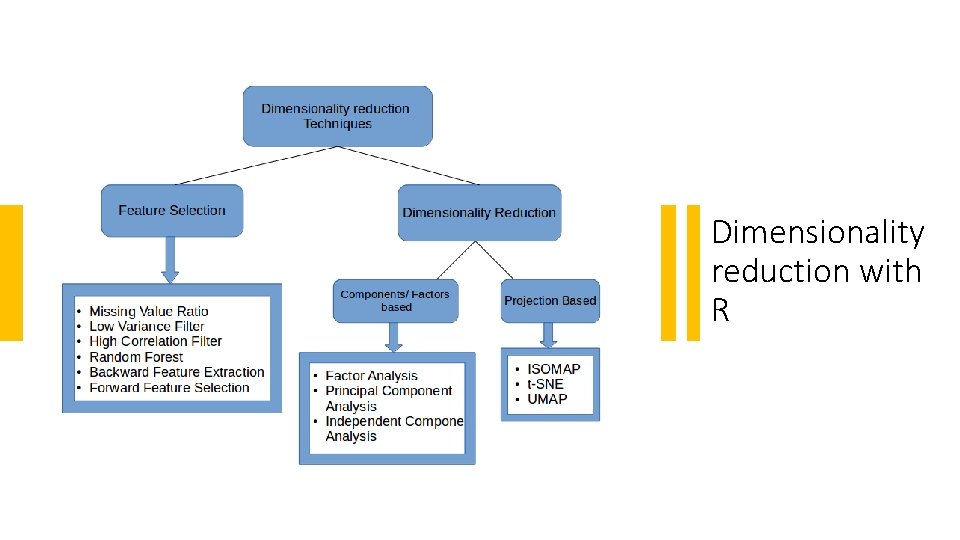
Agenda Dealing with Missing Values • • Test for Missing Values Remove Missing Values Recode Missing Values Exclude Missing Values Dimensionality reduction • • Feature Elimination and Selection Feature Extraction Dimensionality reduction algorithms Exercise: PCA

Why we have to clean data sets? • In general Data science is a blend of three main areas: Mathematics, Technology and Business strategy. • Mathematics is the heart and core of Data science. • Before you apply any algorithm on your data, it is obvious that the data should be tidy or structured. • In the real world, the data are mostly unstructured. • In order to make it tidy and to further apply any algorithm to derive the insights, data has to be cleaned. • The major reason why the data is not tidy is because of the presence of missing values and outliers.

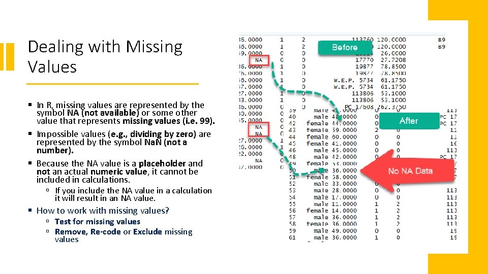
Dealing with Missing Values § In R, missing values are represented by the symbol NA (not available) or some other value that represents missing values (i. e. 99). § Impossible values (e. g. , dividing by zero) are represented by the symbol Na. N (not a number). § Because the NA value is a placeholder and not an actual numeric value, it cannot be included in calculations. ú If you include the NA value in a calculation it will result in an NA value. § How to work with missing values? ú Test for missing values ú Remove, Re-code or Exclude missing values

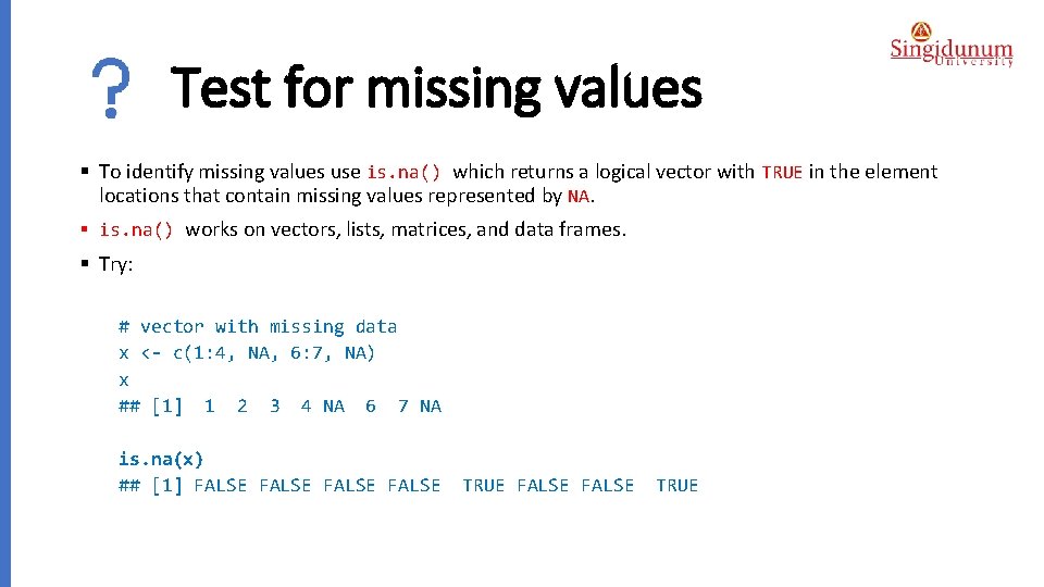
Test for missing values § To identify missing values use is. na() which returns a logical vector with TRUE in the element locations that contain missing values represented by NA. § is. na() works on vectors, lists, matrices, and data frames. § Try: # vector with missing data x <- c(1: 4, NA, 6: 7, NA) x ## [1] 1 2 3 4 NA 6 7 NA is. na(x) ## [1] FALSE TRUE FALSE TRUE

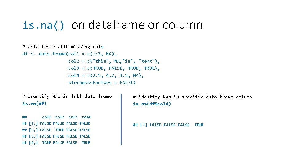
is. na() on dataframe or column # data frame with missing data df <- data. frame(col 1 = c(1: 3, NA), col 2 = c("this", NA, "is", "text"), col 3 = c(TRUE, FALSE, TRUE), col 4 = c(2. 5, 4. 2, 3. 2, NA), strings. As. Factors = FALSE) # identify NAs in full data frame is. na(df) ## col 1 col 2 col 3 col 4 ## [1, ] FALSE ## [2, ] FALSE TRUE FALSE ## [3, ] FALSE ## [4, ] TRUE FALSE # identify NAs in specific data frame column is. na(df$col 4) TRUE ## [1] FALSE TRUE

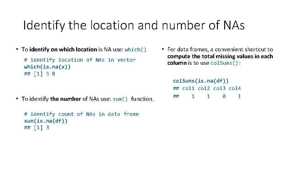
Identify the location and number of NAs • To identify on which location is NA use: which() # identify location of NAs in vector which(is. na(x)) ## [1] 5 8 • To identify the number of NAs use: sum() function. # identify count of NAs in data frame sum(is. na(df)) ## [1] 3 • For data frames, a convenient shortcut to compute the total missing values in each column is to use col. Sums(): col. Sums(is. na(df)) ## col 1 col 2 col 3 col 4 ## 1 1 0 1

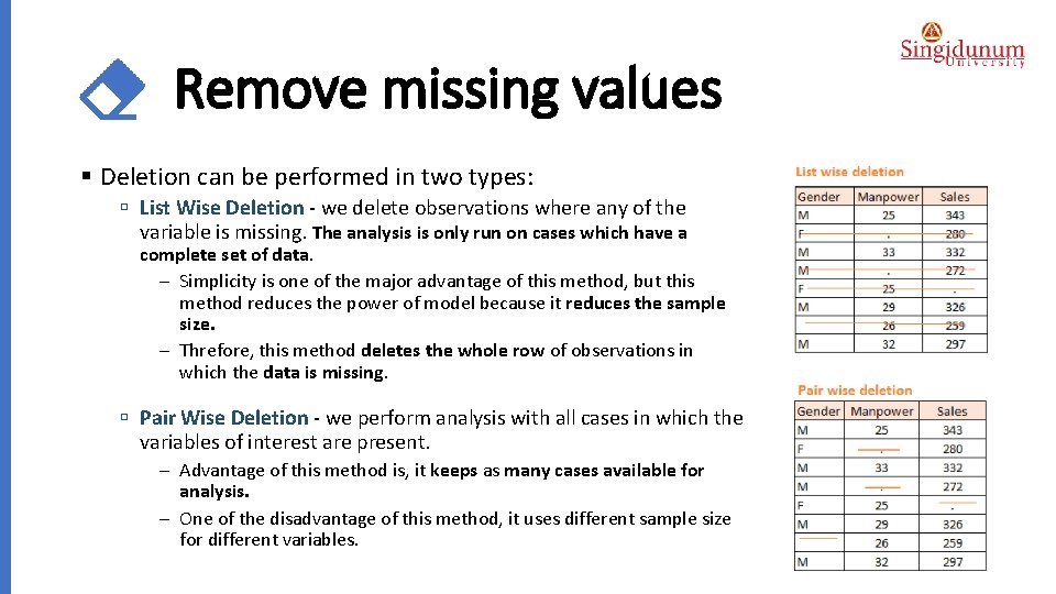
Remove missing values § Deletion can be performed in two types: ú List Wise Deletion - we delete observations where any of the variable is missing. The analysis is only run on cases which have a complete set of data. - Simplicity is one of the major advantage of this method, but this method reduces the power of model because it reduces the sample size. - Threfore, this method deletes the whole row of observations in which the data is missing. ú Pair Wise Deletion - we perform analysis with all cases in which the variables of interest are present. - Advantage of this method is, it keeps as many cases available for analysis. - One of the disadvantage of this method, it uses different sample size for different variables.

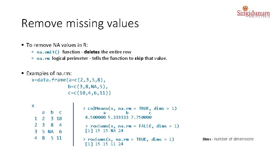
Remove missing values § To remove NA values in R: ú na. omit() function - deletes the entire row ú na. rm logical perimeter - tells the function to skip that value. § Examples of na. rm: x=data. frame(a=c(2, 3, 5, 8), b=c(3, 8, NA, 5), c=c(10, 4, 6, 11)) x 1 2 3 4 a b c 2 3 10 3 8 4 5 NA 6 8 5 11 > col. Means(x, na. rm = TRUE, dims = 1) a b c 4. 500000 5. 333333 7. 750000 > row. Sums(x, na. rm = FALSE, dims = 1) [1] 15 15 NA 24 > row. Sums(x, na. rm = TRUE, dims = 1) [1] 15 15 11 24 Dims - number of dimensions

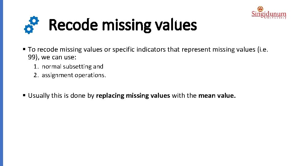
Recode missing values § To recode missing values or specific indicators that represent missing values (i. e. 99), we can use: 1. normal subsetting and 2. assignment operations. § Usually this is done by replacing missing values with the mean value.

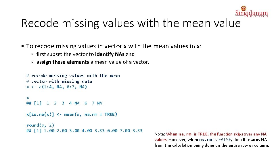
Recode missing values with the mean value § To recode missing values in vector x with the mean values in x: ú first subset the vector to identify NAs and ú assign these elements a mean value of a vector. # recode missing values with the mean # vector with missing data x <- c(1: 4, NA, 6: 7, NA) x ## [1] 1 2 3 4 NA 6 7 NA x[is. na(x)] <- mean(x, na. rm = TRUE) round(x, 2) ## [1] 1. 00 2. 00 3. 00 4. 00 3. 83 6. 00 7. 00 3. 83 Note: When na. rm is TRUE, the function skips over any NA values. However, when na. rm is FALSE, then it returns NA from the calculation being done on the entire row or column.

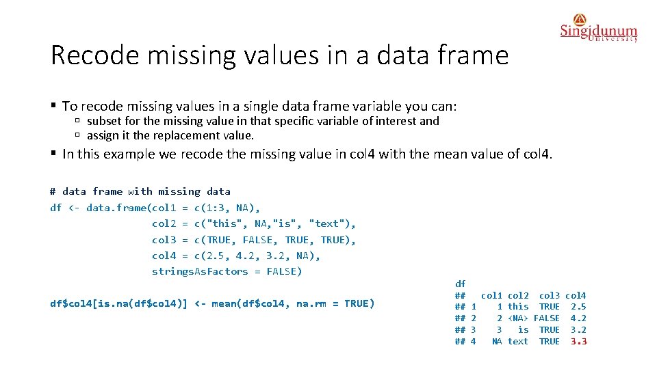
Recode missing values in a data frame § To recode missing values in a single data frame variable you can: ú subset for the missing value in that specific variable of interest and ú assign it the replacement value. § In this example we recode the missing value in col 4 with the mean value of col 4. # data frame with missing data df <- data. frame(col 1 = c(1: 3, NA), col 2 = c("this", NA, "is", "text"), col 3 = c(TRUE, FALSE, TRUE), col 4 = c(2. 5, 4. 2, 3. 2, NA), strings. As. Factors = FALSE) df$col 4[is. na(df$col 4)] <- mean(df$col 4, na. rm = TRUE) df ## ## ## 1 2 3 4 col 1 1 2 3 NA col 2 col 3 col 4 this TRUE 2. 5 <NA> FALSE 4. 2 is TRUE 3. 2 text TRUE 3. 3

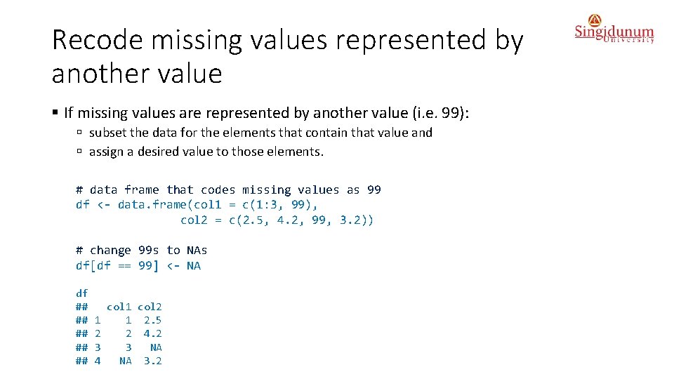
Recode missing values represented by another value § If missing values are represented by another value (i. e. 99): ú subset the data for the elements that contain that value and ú assign a desired value to those elements. # data frame that codes missing values as 99 df <- data. frame(col 1 = c(1: 3, 99), col 2 = c(2. 5, 4. 2, 99, 3. 2)) # change 99 s to NAs df[df == 99] <- NA df ## ## ## 1 2 3 4 col 1 col 2 1 2. 5 2 4. 2 3 NA NA 3. 2

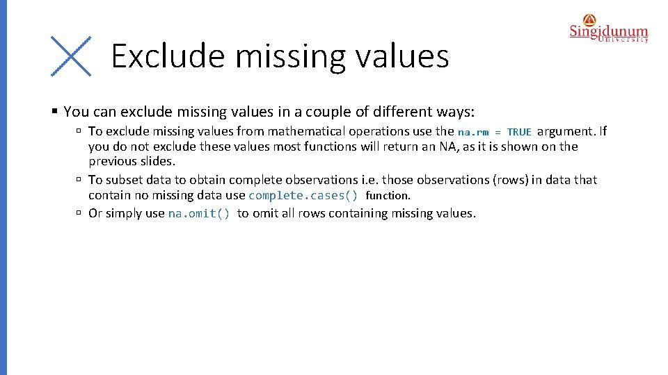
Exclude missing values § You can exclude missing values in a couple of different ways: ú To exclude missing values from mathematical operations use the na. rm = TRUE argument. If you do not exclude these values most functions will return an NA, as it is shown on the previous slides. ú To subset data to obtain complete observations i. e. those observations (rows) in data that contain no missing data use complete. cases() function. ú Or simply use na. omit() to omit all rows containing missing values.

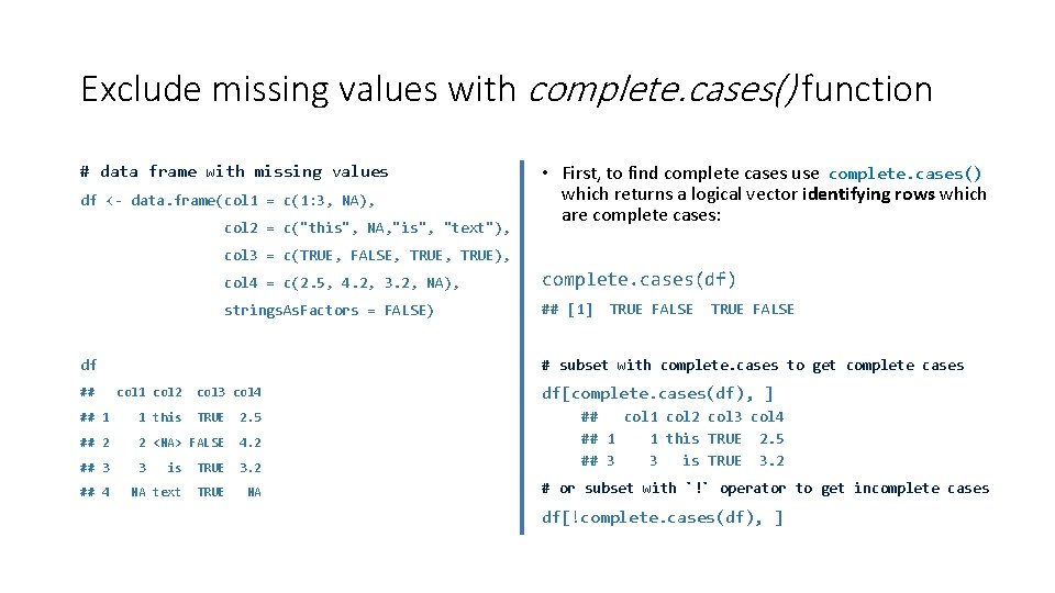
Exclude missing values with complete. cases() function # data frame with missing values df <- data. frame(col 1 = c(1: 3, NA), col 2 = c("this", NA, "is", "text"), • First, to find complete cases use complete. cases() which returns a logical vector identifying rows which are complete cases: col 3 = c(TRUE, FALSE, TRUE), col 4 = c(2. 5, 4. 2, 3. 2, NA), complete. cases(df) strings. As. Factors = FALSE) ## [1] col 1 col 2 col 3 col 4 ## 1 1 this TRUE 2. 5 ## 2 2 <NA> FALSE 4. 2 ## 3 3 ## 4 TRUE FALSE # subset with complete. cases to get complete cases df ## TRUE FALSE is TRUE 3. 2 NA text TRUE NA df[complete. cases(df), ] ## col 1 col 2 col 3 col 4 ## 1 1 this TRUE 2. 5 ## 3 3 is TRUE 3. 2 # or subset with `!` operator to get incomplete cases df[!complete. cases(df), ]

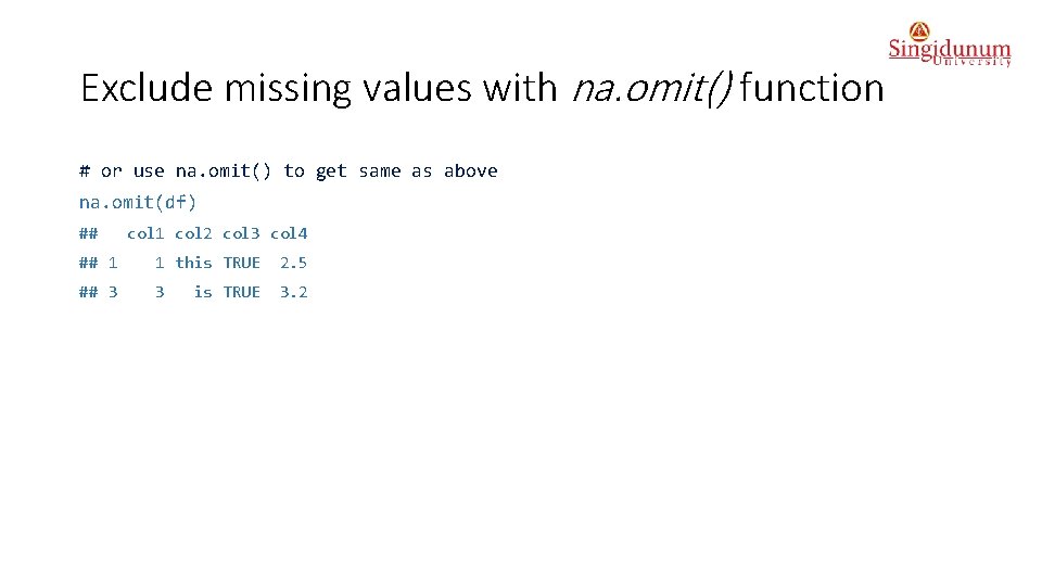
Exclude missing values with na. omit() function # or use na. omit() to get same as above na. omit(df) ## col 1 col 2 col 3 col 4 ## 1 1 this TRUE 2. 5 ## 3 3 3. 2 is TRUE

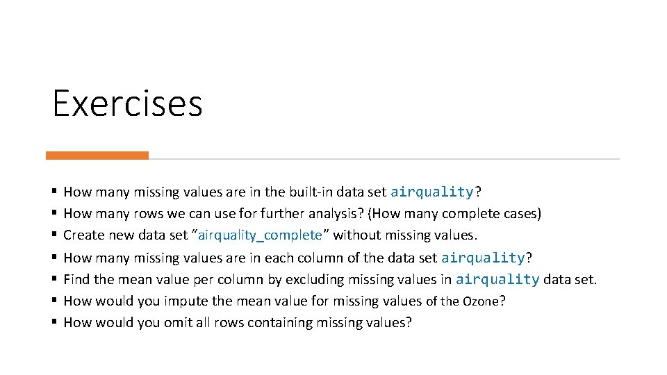
Exercises § § § § How many missing values are in the built-in data set airquality? How many rows we can use for further analysis? (How many complete cases) Create new data set “airquality_complete” without missing values. How many missing values are in each column of the data set airquality? Find the mean value per column by excluding missing values in airquality data set. How would you impute the mean value for missing values of the Ozone? How would you omit all rows containing missing values?

Solution § How many missing values are in the built-in data set airquality? # Load and inspect data(airquality) # Load the data set airquality dim(airquality) # The dim function returns the dimension (e. g. the number of columns and rows). head(airquality) # Head of data # How many missing values sum(is. na(airquality))

Solution § How many rows we can use for further analysis? (How many complete cases) sum(complete. cases(airquality)) # Another way dim(na. omit(airquality)) § Create new data set “airquality_complete” without missing values: airquality_complete=airquality[complete. cases(airquality), ] # Check is there any NAs sum(is. na(airquality_complete))

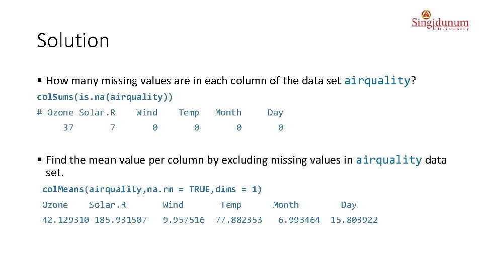
Solution § How many missing values are in each column of the data set airquality? col. Sums(is. na(airquality)) # Ozone Solar. R 37 Wind Temp Month Day 0 0 7 § Find the mean value per column by excluding missing values in airquality data set. col. Means(airquality, na. rm = TRUE, dims = 1) Ozone Solar. R 42. 129310 185. 931507 Wind 9. 957516 Temp 77. 882353 Month 6. 993464 Day 15. 803922

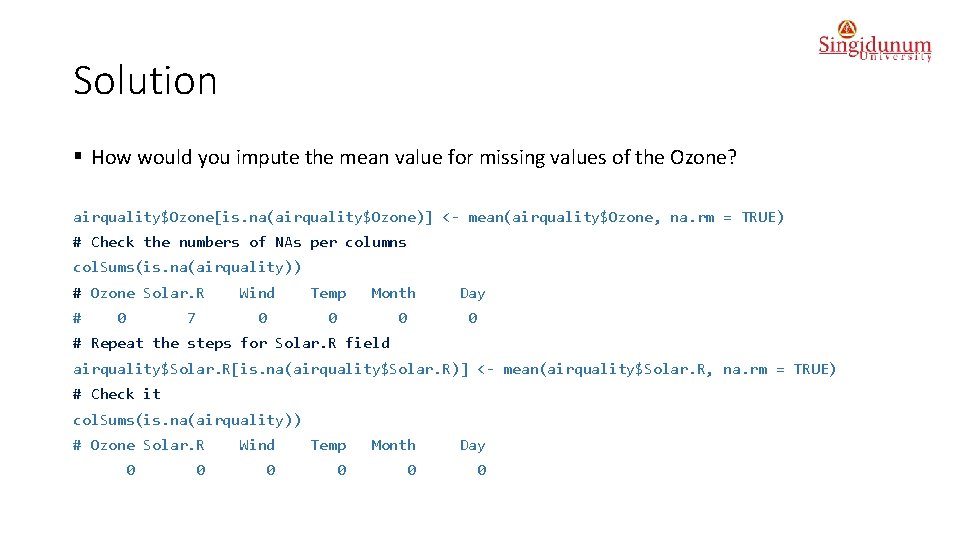
Solution § How would you impute the mean value for missing values of the Ozone? airquality$Ozone[is. na(airquality$Ozone)] <- mean(airquality$Ozone, na. rm = TRUE) # Check the numbers of NAs per columns col. Sums(is. na(airquality)) # Ozone Solar. R # 0 7 Wind Temp 0 0 Month 0 Day 0 # Repeat the steps for Solar. R field airquality$Solar. R[is. na(airquality$Solar. R)] <- mean(airquality$Solar. R, na. rm = TRUE) # Check it col. Sums(is. na(airquality)) # Ozone Solar. R 0 0 Wind Temp Month Day 0 0

Solution § How would you omit all rows containing missing values? na. omit(airquality)

Dimensionality reduction with R

Why we need to reduce dimensionality? § Dealing with a lot of dimensions can be painful for machine learning algorithms. § High dimensionality will increase: ú the computational complexity ú the risk of overfitting ú the sparsity of the data. § Dimensionality reduction will project the data in a space with less dimension to limit these phenomena.

What is dimension reduction? § Dimension reduction is the process of reducing the number of variables (features, dimensions) to a set of values of variables called principal variables. § The main properties of principal variables are: ú preservation of the structure and information carried by the original variables, to some extent. ú Principal variables are ordered by importance, with the first variable preserving the most structure and following variables preserving successively less. § In other words applying dimension reduction to a data set creates a data set with the same number of observations but less variables, whilst maintaining the general “flavor” of the data set.

Dimension reduction techniques § There are many different dimension reduction techniques that all try to find a representation of the data in a lower dimensional space that retains as much information as possible. § In general there are two classes of dimension reduction: ú Feature Elimination and Selection is removing some variables completely if they are redundant with some other variable or if they are not providing any new information about the data set. - The advantage of feature elimination is that it is simple to implement and makes our data set small, including only variables in which we are interested. - But as a disadvantage — we might lose some information from the variables which we dropped. ú Feature Extraction on the other hand, is the formation of new variables from the old variables. - The advantage of feature extraction is that it preserves the most structure of your original data set. - But as a disadvantage - the newly created variables loose their interpretation.

Features selection § The most obvious way to reduce dimensionality is to remove some dimensions and to select the more suitable variables for the problem. § Here are some ways to select variables: ú Greedy algorithms which add and remove variables until some criterion is met. For instance, the stepwise regression with forward selection will add at each step the variable which improve the fit in the most significant way ú Shrinking and penalization methods, which will add cost for having too many variables. For instance, L 1 regularization will cut some variables’ coefficient to zero. Regularization limits the space where the coefficients can live in. ú Selection of models based on criteria taking the number of dimensions into accounts. Contrary to regularization, the model is not trained to optimize these criteria. The criteria are computed after fitting to compare several models. ú Filtering of variables using correlation or some “distance measure” between the features.

Feature extraction § Dimension reduction via feature extraction is an extremely powerful statistical tool and thus is frequently applied. § Features extraction (or engineering) seeks to keep only the intervals or modalities of the features which contain information. § Some of the main uses of dimension reduction are: ú simplification ú denoising ú variable selection ú visualization

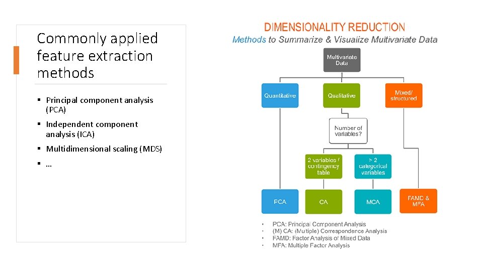
Commonly applied feature extraction methods § Principal component analysis (PCA) § Independent component analysis (ICA) § Multidimensional scaling (MDS) § …

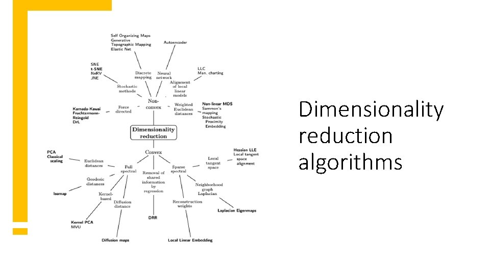
Dimensionality reduction algorithms

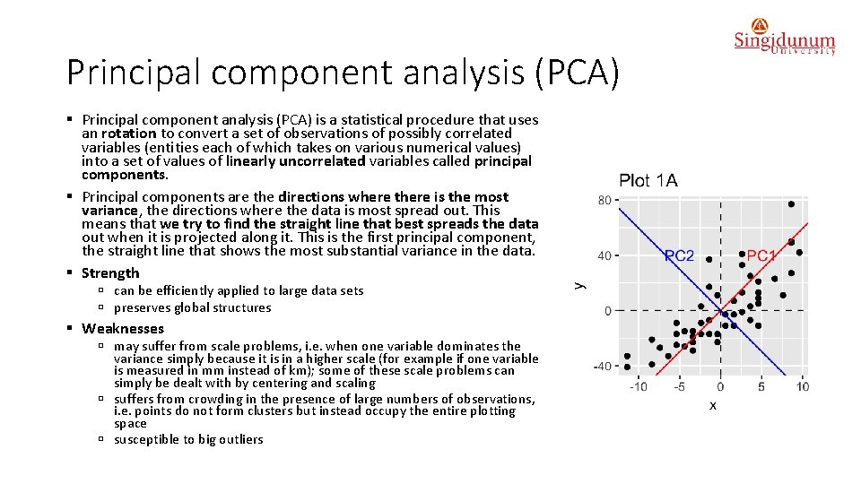
Principal component analysis (PCA) § Principal component analysis (PCA) is a statistical procedure that uses an rotation to convert a set of observations of possibly correlated variables (entities each of which takes on various numerical values) into a set of values of linearly uncorrelated variables called principal components. § Principal components are the directions where there is the most variance, the directions where the data is most spread out. This means that we try to find the straight line that best spreads the data out when it is projected along it. This is the first principal component, the straight line that shows the most substantial variance in the data. § Strength ú can be efficiently applied to large data sets ú preserves global structures § Weaknesses ú may suffer from scale problems, i. e. when one variable dominates the variance simply because it is in a higher scale (for example if one variable is measured in mm instead of km); some of these scale problems can simply be dealt with by centering and scaling ú suffers from crowding in the presence of large numbers of observations, i. e. points do not form clusters but instead occupy the entire plotting space ú susceptible to big outliers

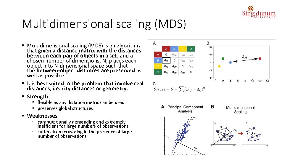
Multidimensional scaling (MDS) § Multidimensional scaling (MDS) is an algorithm that given a distance matrix with the distances between each pair of objects in a set, and a chosen number of dimensions, N, places each object into N-dimensional space such that the between-object distances are preserved as well as possible. § It is best suited to the problem that involve real distances, i. e. city distances or geometry. § Strength ú flexible as any distance metric can be used ú preserves global structures § Weaknesses ú computationally demanding and extremely inefficient for large numbers of observations ú suffers from crowding in the presence of large number of observations

Independent component analysis (ICA) § Independent component analysis (ICA) attempts to decompose a multivariate signal into statistically independent non-Gaussian signals. § ICA is important to blind signal separation and has many practical applications but the most common is applications for sound signals. § A simple application of ICA is the “cocktail party problem”, where the underlying speech signals are separated from a sample data consisting of people talking simultaneously in a room. ú Usually the problem is simplified by assuming no time delays or echoes. ú Note that a filtered and delayed signal is a copy of a dependent component, and thus the statistical independence assumption is not violated. § Strength ú separating multiple independent sources of signal ú can be efficiently applied to large data sets ú preserves global structures § Weaknesses ú has very specific assumptions, especially that none of the independent sources are normally distributed ú suffers from crowding in the presence of large number of observations

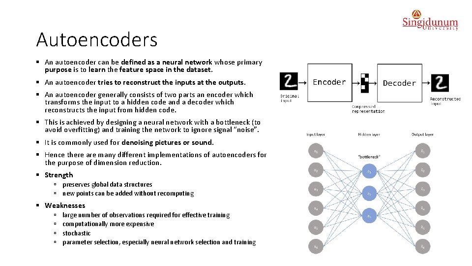
Autoencoders § An autoencoder can be defined as a neural network whose primary purpose is to learn the feature space in the dataset. § An autoencoder tries to reconstruct the inputs at the outputs. § An autoencoder generally consists of two parts an encoder which transforms the input to a hidden code and a decoder which reconstructs the input from hidden code. § This is achieved by designing a neural network with a bottleneck (to avoid overfitting) and training the network to ignore signal “noise”. § It is commonly used for denoising pictures or sound. § Hence there are many different implementations of autoencoders for the purpose of dimension reduction. § Strength ú preserves global data structures ú new points can be added without recomputing § Weaknesses ú ú large number of observations required for effective training computationally more expensive stochastic parameter selection, especially neural network selection and training

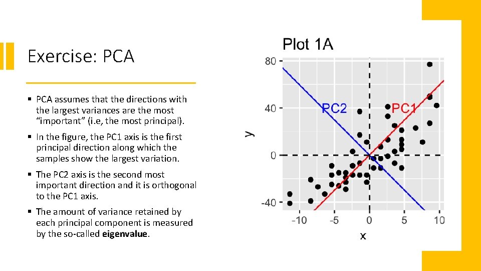
Exercise: PCA § PCA assumes that the directions with the largest variances are the most “important” (i. e, the most principal). § In the figure, the PC 1 axis is the first principal direction along which the samples show the largest variation. § The PC 2 axis is the second most important direction and it is orthogonal to the PC 1 axis. § The amount of variance retained by each principal component is measured by the so-called eigenvalue.

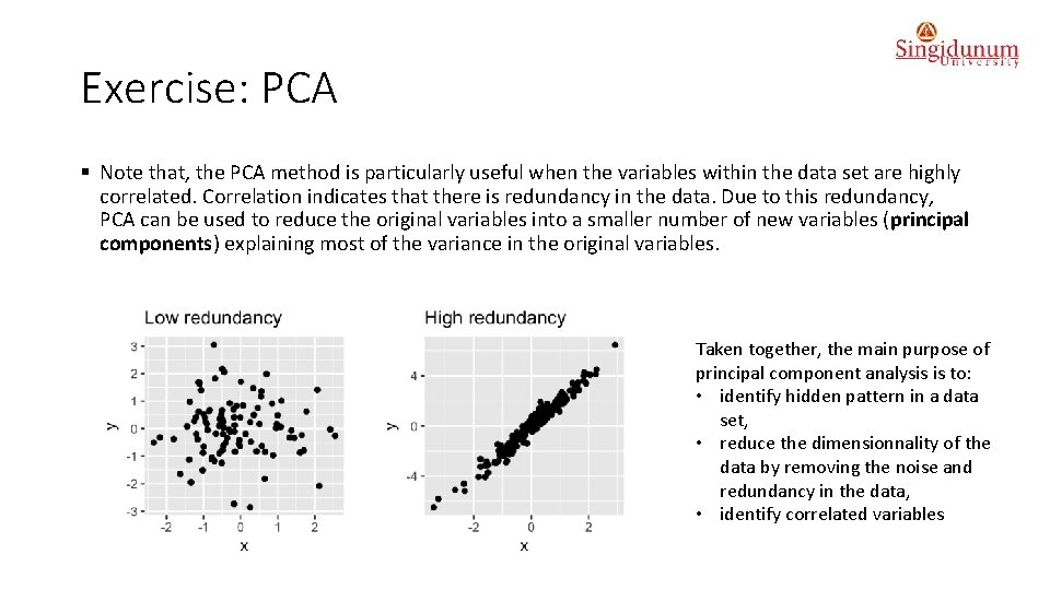
Exercise: PCA § Note that, the PCA method is particularly useful when the variables within the data set are highly correlated. Correlation indicates that there is redundancy in the data. Due to this redundancy, PCA can be used to reduce the original variables into a smaller number of new variables (principal components) explaining most of the variance in the original variables. Taken together, the main purpose of principal component analysis is to: • identify hidden pattern in a data set, • reduce the dimensionnality of the data by removing the noise and redundancy in the data, • identify correlated variables

R packages for PCA § Several functions from different packages are available in the R software for computing PCA: ú ú prcomp() and princomp() [built-in R stats package], PCA() [Facto. Mine. R package], dudi. pca() [ade 4 package], ep. PCA() [Ex. Position package] § No matter what function you decide to use, you can easily extract and visualize the results of PCA using R functions provided in the factoextra R package. § In this exercise we will use the two packages Facto. Mine. R (for the analysis) and factoextra (for ggplot 2 -based visualization).

Step 1. Install packages for PCA #Install the two packages as follow: install. packages(c("Facto. Mine. R", "factoextra")) # Load them in R, by typing this: library("Facto. Mine. R") library("factoextra")

Step 2: Import dataset § Download “Decathlon. csv” dataset: https: //www. kaggle. com/dhafer/decathlon § Dataset describes athletes’ performance during two sporting events (Desctar and Olympic. G). § It contains 27 individuals (athletes) described by 13 variables. data(decathlon) head(decathlon)

Step 3: Subset rows and columns for PCA for train and test § Only some of these individuals and variables will be used to perform the PCA analysis. The coordinates of the remaining individuals and variables on the factor map will be predicted after the PCA. § Dataset will be divided as: ú Rows will be divided: - First 23 individuals will be used for PCA - The last 4 rows (rows 24: 27) will be predicted using the PCA and parameters obtained with analysed individuals ú Columns (variables) will be divided: - First 10 variables (columns 1: 10) will be used for PCA analysis. - Columns 11: 12 which correspond to the rank and the points of athletes will be predicted. - Column 13 is categorical (factor) value which corresponds to the two athlete meetings (Olympic Game and Decastar) – this column will be used to color individuals by groups. decathlon 2. active <- decathlon[1: 23, 1: 10] head(decathlon 2. active[, 1: 6], 4)

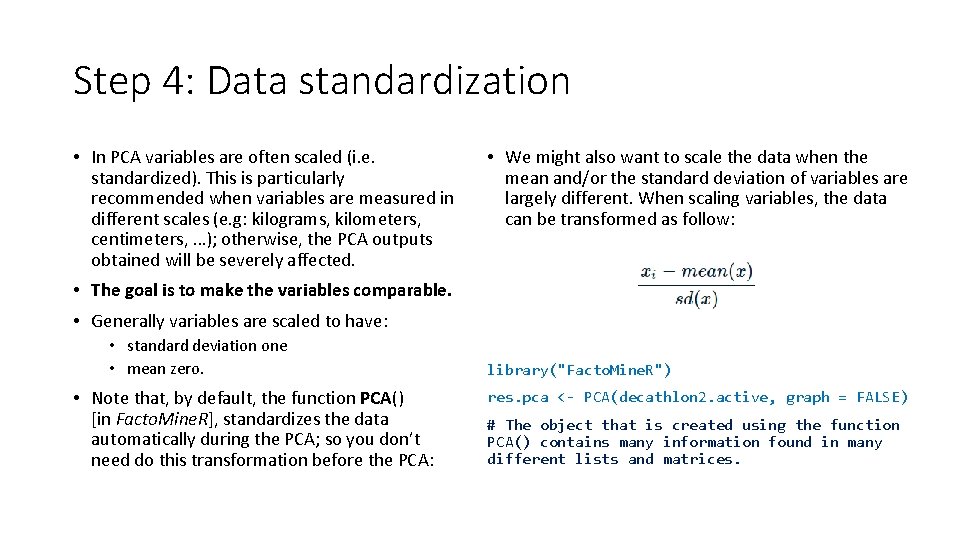
Step 4: Data standardization • In PCA variables are often scaled (i. e. standardized). This is particularly recommended when variables are measured in different scales (e. g: kilograms, kilometers, centimeters, …); otherwise, the PCA outputs obtained will be severely affected. • We might also want to scale the data when the mean and/or the standard deviation of variables are largely different. When scaling variables, the data can be transformed as follow: • The goal is to make the variables comparable. • Generally variables are scaled to have: • standard deviation one • mean zero. • Note that, by default, the function PCA() [in Facto. Mine. R], standardizes the data automatically during the PCA; so you don’t need do this transformation before the PCA: library("Facto. Mine. R") res. pca <- PCA(decathlon 2. active, graph = FALSE) # The object that is created using the function PCA() contains many information found in many different lists and matrices.

Step 5: Visualize and interpret § No matter what function you decide to use [stats: : prcomp(), Facto. Miner: : PCA(), ade 4: : dudi. pca(), Ex. Position: : ep. PCA()], you can easily extract and visualize the results of PCA using R functions provided in the factoextra R package. § We’ll use the factoextra R package to help in the interpretation of PCA. § These functions include: ú get_eigenvalue(res. pca): Extract the eigenvalues/variances of principal components ú fviz_eig(res. pca): Visualize the eigenvalues ú get_pca_ind(res. pca), get_pca_var(res. pca): Extract the results for individuals and variables, respectively. ú fviz_pca_ind(res. pca), fviz_pca_var(res. pca): Visualize the results individuals and variables, respectively. ú fviz_pca_biplot(res. pca): Make a biplot of individuals and variables. § On the next slides these functions will be demonstrated.

Eigenvalues / Variances § The eigenvalues measure the amount of variation retained by each principal component. § Eigenvalues are large for the first Principal Components (PCs) and small for the subsequent PCs. That is, the first PCs corresponds to the directions with the maximum amount of variation in the data set. § We examine the eigenvalues to determine the number of principal components to be considered. § The eigenvalues and the proportion of variances (i. e. , information) retained by the PCs can be extracted using the function get_eigenvalue() [factoextra package]. library("factoextra") eig. val <- get_eigenvalue(res. pca) eig. val

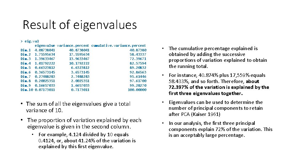
Result of eigenvalues > eig. val eigenvalue variance. percent cumulative. variance. percent Dim. 1 4. 08738041 40. 87380 Dim. 2 1. 75595634 17. 5595634 58. 43337 Dim. 3 1. 39633467 13. 9633467 72. 39671 Dim. 4 1. 01792222 10. 1792222 82. 57594 Dim. 5 0. 66323812 6. 6323812 89. 20832 Dim. 6 0. 36573145 3. 6573145 92. 86563 Dim. 7 0. 27488283 2. 7488283 95. 61446 Dim. 8 0. 20025351 2. 0025351 97. 61700 Dim. 9 0. 16657033 1. 6657033 99. 28270 Dim. 10 0. 07173011 0. 7173011 100. 00000 • The sum of all the eigenvalues give a total variance of 10. • The proportion of variation explained by each eigenvalue is given in the second column. • For example, 4. 124 divided by 10 equals 0. 4124, or, about 41. 24% of the variation is explained by this first eigenvalue. • The cumulative percentage explained is obtained by adding the successive proportions of variation explained to obtain the running total. • For instance, 40. 874% plus 17, 559% equals 58. 433%, and so forth. Therefore, about 72. 397% of the variation is explained by the first three eigenvalues together. • Eigenvalues can be used to determine the number of principal components to retain after PCA (Kaiser 1961) • In our analysis, the first three principal components explain 72% of the variation. This is an acceptably large percentage.

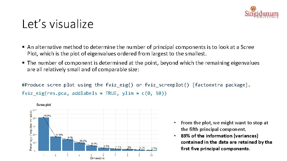
Let’s visualize § An alternative method to determine the number of principal components is to look at a Scree Plot, which is the plot of eigenvalues ordered from largest to the smallest. § The number of component is determined at the point, beyond which the remaining eigenvalues are all relatively small and of comparable size: #Produce scree plot using the fviz_eig() or fviz_screeplot() [factoextra package]. fviz_eig(res. pca, addlabels = TRUE, ylim = c(0, 50)) • From the plot, we might want to stop at the fifth principal component. • 89% of the information (variances) contained in the data are retained by the first five principal components.

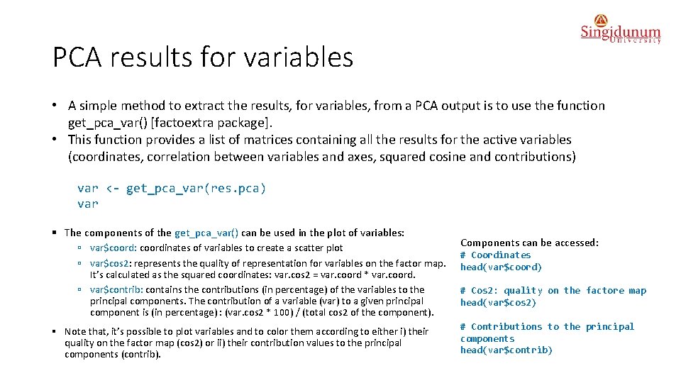
PCA results for variables • A simple method to extract the results, for variables, from a PCA output is to use the function get_pca_var() [factoextra package]. • This function provides a list of matrices containing all the results for the active variables (coordinates, correlation between variables and axes, squared cosine and contributions) var <- get_pca_var(res. pca) var § The components of the get_pca_var() can be used in the plot of variables: ú var$coord: coordinates of variables to create a scatter plot ú var$cos 2: represents the quality of representation for variables on the factor map. It’s calculated as the squared coordinates: var. cos 2 = var. coord * var. coord. ú var$contrib: contains the contributions (in percentage) of the variables to the principal components. The contribution of a variable (var) to a given principal component is (in percentage) : (var. cos 2 * 100) / (total cos 2 of the component). § Note that, it’s possible to plot variables and to color them according to either i) their quality on the factor map (cos 2) or ii) their contribution values to the principal components (contrib). Components can be accessed: # Coordinates head(var$coord) # Cos 2: quality on the factore map head(var$cos 2) # Contributions to the principal components head(var$contrib)

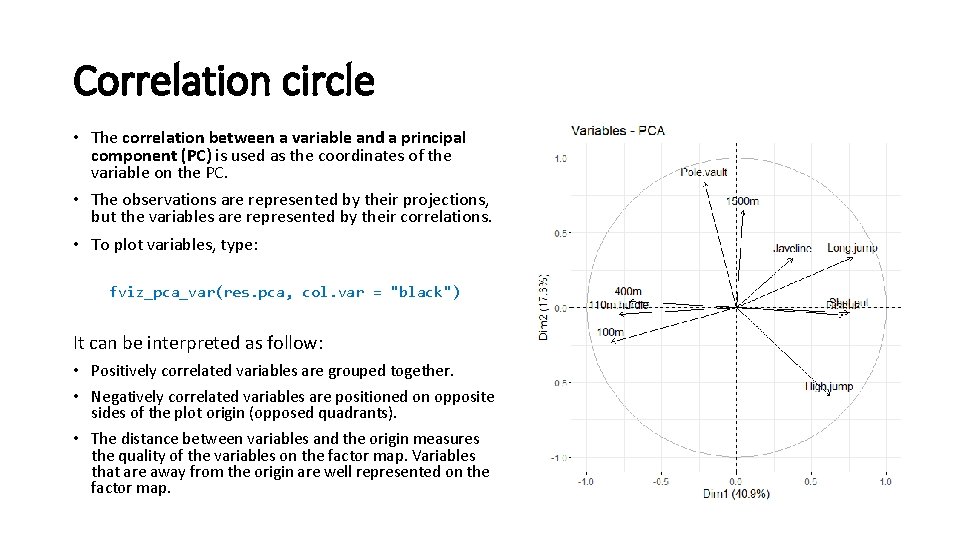
Correlation circle • The correlation between a variable and a principal component (PC) is used as the coordinates of the variable on the PC. • The observations are represented by their projections, but the variables are represented by their correlations. • To plot variables, type: fviz_pca_var(res. pca, col. var = "black") It can be interpreted as follow: • Positively correlated variables are grouped together. • Negatively correlated variables are positioned on opposite sides of the plot origin (opposed quadrants). • The distance between variables and the origin measures the quality of the variables on the factor map. Variables that are away from the origin are well represented on the factor map.

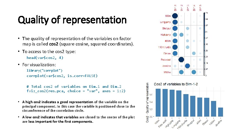
Quality of representation • The quality of representation of the variables on factor map is called cos 2 (square cosine, squared coordinates). • To access to the cos 2 type: head(var$cos 2, 4) • For visualization: library("corrplot") corrplot(var$cos 2, is. corr=FALSE) # Total cos 2 of variables on Dim. 1 and Dim. 2 fviz_cos 2(res. pca, choice = "var", axes = 1: 2) • A high cos 2 indicates a good representation of the variable on the principal component. In this case the variable is positioned close to the circumference of the correlation circle. • A low cos 2 indicates that variables are closed to the center of the plot are less important for the first components.

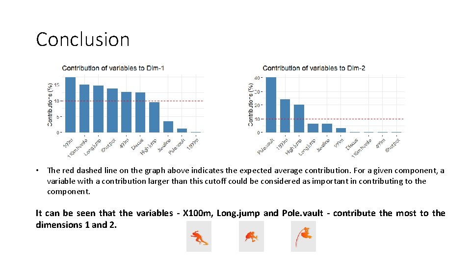
Contributions of variables to PCs § Variables that are correlated with PC 1 (i. e. , Dim. 1) and PC 2 (i. e. , Dim. 2) are the most important in explaining the variability in the data set. § Variables that do not correlated with any PC or correlated with the last dimensions are variables with low contribution and might be removed to simplify the overall analysis. § The contribution of variables can be extracted as: head(var$contrib, 4) § The larger the value of the contribution, the more the variable contributes to the component. Let’s visualize that: # Contributions of variables fviz_contrib(res. pca, choice to PC 1 = "var", axes = 1, top = 10) to PC 2 = "var", axes = 2, top = 10)

Conclusion • The red dashed line on the graph above indicates the expected average contribution. For a given component, a variable with a contribution larger than this cutoff could be considered as important in contributing to the component. It can be seen that the variables - X 100 m, Long. jump and Pole. vault - contribute the most to the dimensions 1 and 2.