CSE 245 ComputerAided Circuit Simulation and Verification Lecture

CSE 245: Computer-Aided Circuit Simulation and Verification Lecture Note 2: State Equations Spring 2010 Prof. Chung-Kuan Cheng

State Equations 1. 2. 3. 4. Motivation Formulation Analytical Solution Frequency Domain Analysis 5. Concept of Moments

Motivation • Why – Whole Circuit Analysis – Interconnect Dominance • Wires smaller R increase • Separation smaller C increase • What – Power Net, Clock, Interconnect Coupling, Parallel Processing • Where – – Matrix Solvers, Integration For Dynamic System RLC Reduction, Transmission Lines, S Parameters Whole Chip Analysis Thermal, Mechanical, Biological Analysis

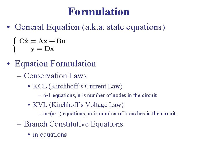
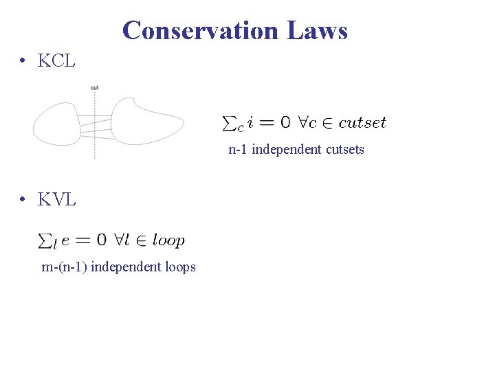
Formulation • General Equation (a. k. a. state equations) • Equation Formulation – Conservation Laws • KCL (Kirchhoff’s Current Law) – n-1 equations, n is number of nodes in the circuit • KVL (Kirchhoff’s Voltage Law) – m-(n-1) equations, m is number of branches in the circuit. – Branch Constitutive Equations • m equations

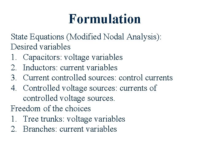
Formulation State Equations (Modified Nodal Analysis): Desired variables 1. Capacitors: voltage variables 2. Inductors: current variables 3. Current controlled sources: control currents 4. Controlled voltage sources: currents of controlled voltage sources. Freedom of the choices 1. Tree trunks: voltage variables 2. Branches: current variables

Conservation Laws • KCL n-1 independent cutsets • KVL m-(n-1) independent loops

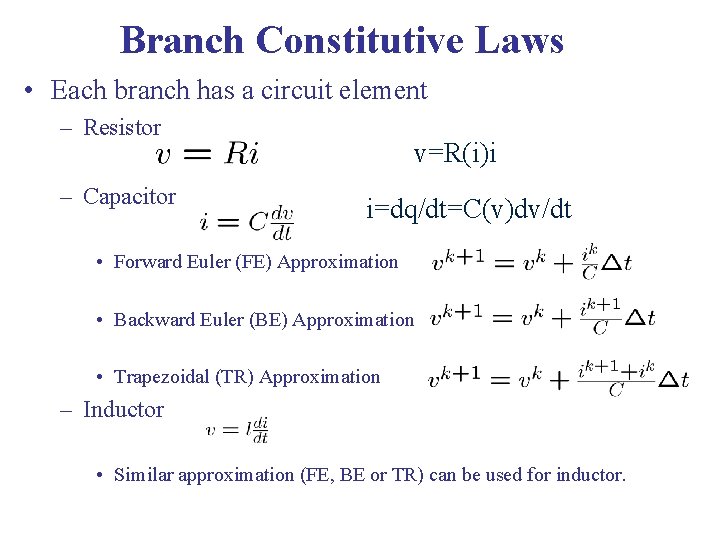
Branch Constitutive Laws • Each branch has a circuit element – Resistor – Capacitor v=R(i)i i=dq/dt=C(v)dv/dt • Forward Euler (FE) Approximation • Backward Euler (BE) Approximation • Trapezoidal (TR) Approximation – Inductor • Similar approximation (FE, BE or TR) can be used for inductor.

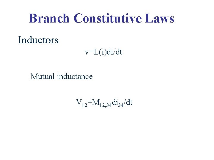
Branch Constitutive Laws Inductors v=L(i)di/dt Mutual inductance V 12=M 12, 34 di 34/dt

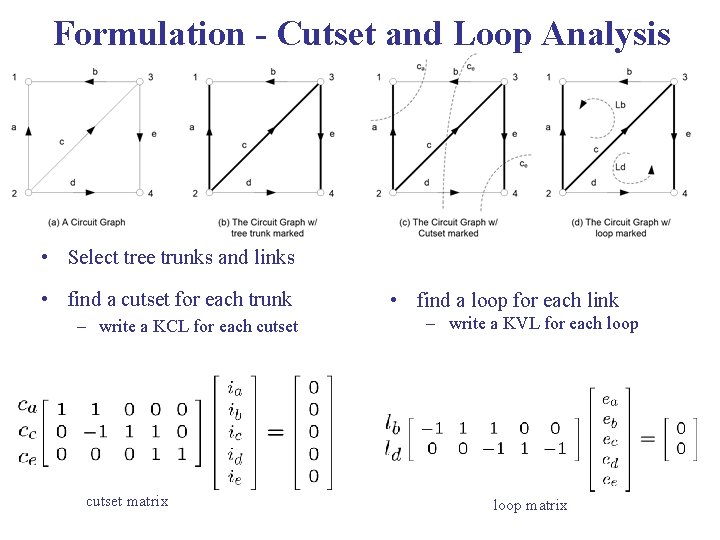
Formulation - Cutset and Loop Analysis • Select tree trunks and links • find a cutset for each trunk – write a KCL for each cutset matrix • find a loop for each link – write a KVL for each loop matrix

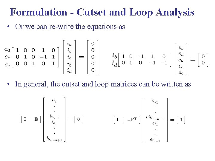
Formulation - Cutset and Loop Analysis • Or we can re-write the equations as: • In general, the cutset and loop matrices can be written as

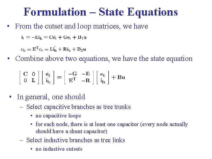
Formulation – State Equations • From the cutset and loop matrices, we have • Combine above two equations, we have the state equation • In general, one should – Select capacitive branches as tree trunks • no capacitive loops • for each node, there is at least one capacitor (every node actually should have a shunt capacitor) – Select inductive branches as tree links • no inductive cutsets

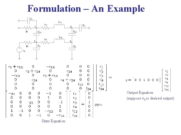
Formulation – An Example Output Equation (suppose v 3 is desired output) State Equation

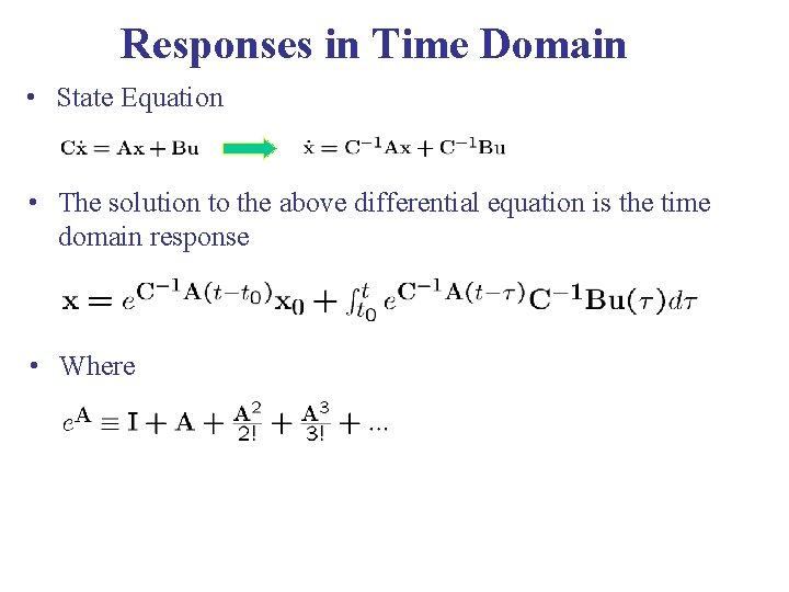
Responses in Time Domain • State Equation • The solution to the above differential equation is the time domain response • Where

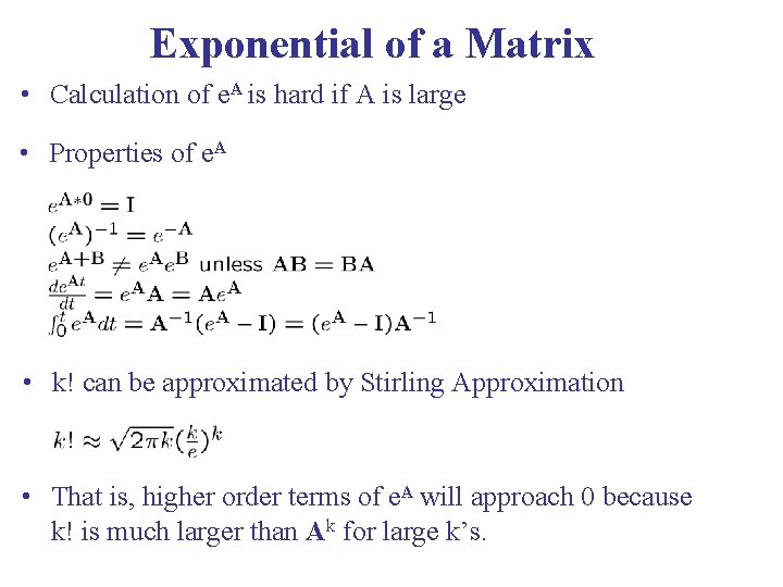
Exponential of a Matrix • Calculation of e. A is hard if A is large • Properties of e. A • k! can be approximated by Stirling Approximation • That is, higher order terms of e. A will approach 0 because k! is much larger than Ak for large k’s.

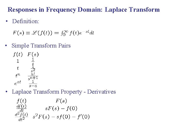
Responses in Frequency Domain: Laplace Transform • Definition: • Simple Transform Pairs • Laplace Transform Property - Derivatives

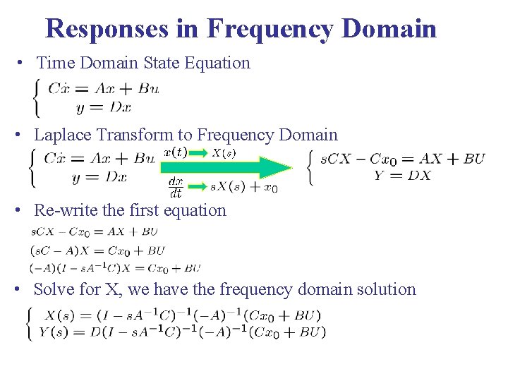
Responses in Frequency Domain • Time Domain State Equation • Laplace Transform to Frequency Domain • Re-write the first equation • Solve for X, we have the frequency domain solution

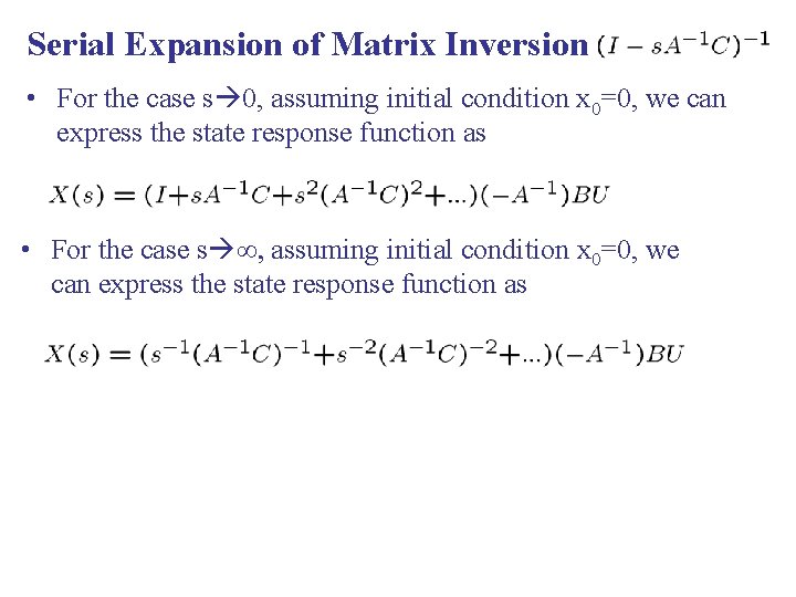
Serial Expansion of Matrix Inversion • For the case s 0, assuming initial condition x 0=0, we can express the state response function as • For the case s , assuming initial condition x 0=0, we can express the state response function as

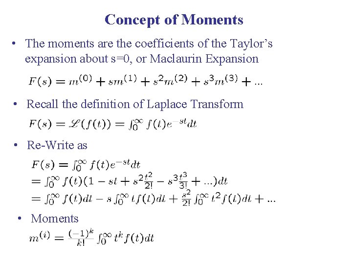
Concept of Moments • The moments are the coefficients of the Taylor’s expansion about s=0, or Maclaurin Expansion • Recall the definition of Laplace Transform • Re-Write as • Moments

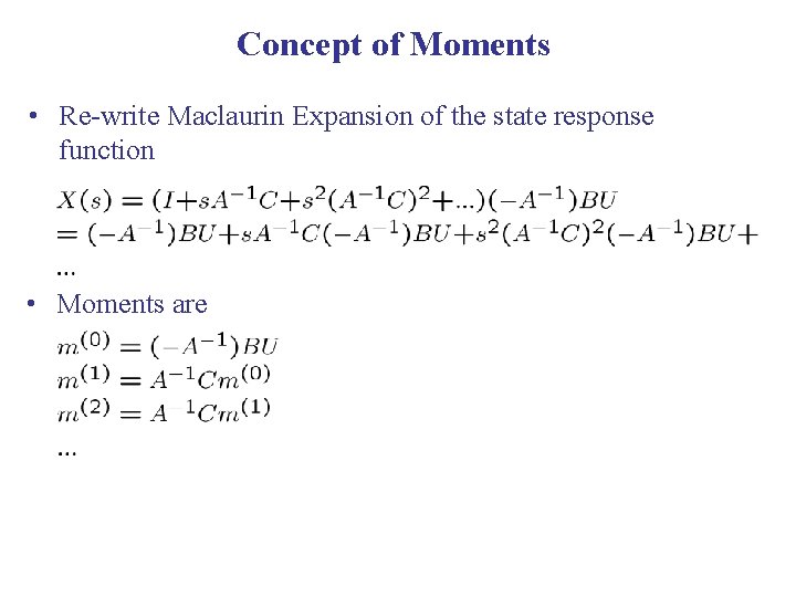
Concept of Moments • Re-write Maclaurin Expansion of the state response function • Moments are

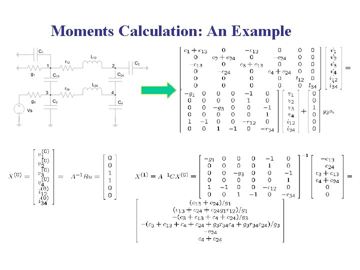
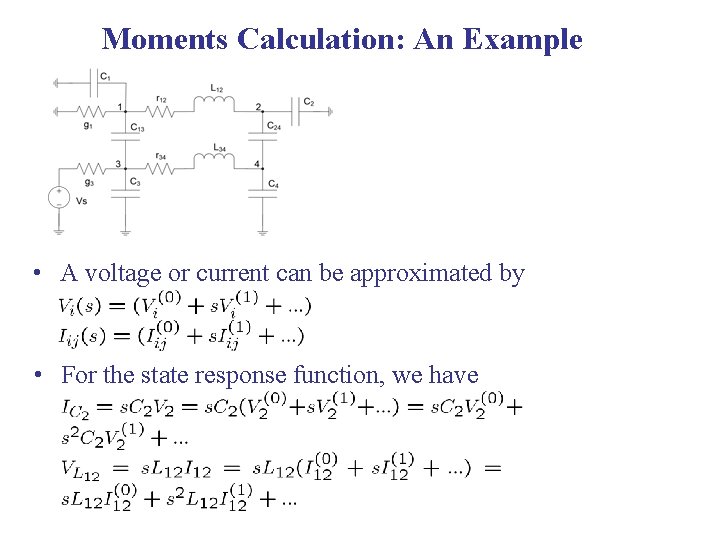
Moments Calculation: An Example

Moments Calculation: An Example • A voltage or current can be approximated by • For the state response function, we have

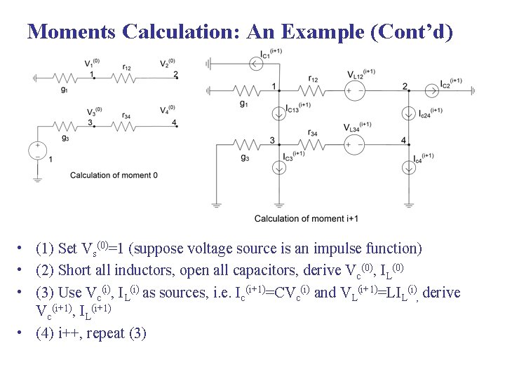
Moments Calculation: An Example (Cont’d) • (1) Set Vs(0)=1 (suppose voltage source is an impulse function) • (2) Short all inductors, open all capacitors, derive Vc(0), IL(0) • (3) Use Vc(i), IL(i) as sources, i. e. Ic(i+1)=CVc(i) and VL(i+1)=LIL(i), derive Vc(i+1), IL(i+1) • (4) i++, repeat (3)