CSE 245 ComputerAided Circuit Simulation and Verification Lecture

CSE 245: Computer-Aided Circuit Simulation and Verification Lecture Notes 3 Model Order Reduction (1) Spring 2006 Prof. Chung-Kuan Cheng UCSD CSE 245 Notes – SPRING 2006

Outline • Introduction • Formulation • Linear System – Time Domain Analysis – Frequency Domain Analysis – Moments – Stability and Passivity – Model Order Reduction UCSD CSE 245 Notes – SPRING 2006

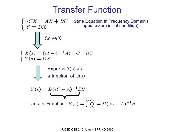
Transfer Function State Equation in Frequency Domain ( suppose zero initial condition) Solve X Express Y(s) as a function of U(s) Transfer Function: UCSD CSE 245 Notes – SPRING 2006

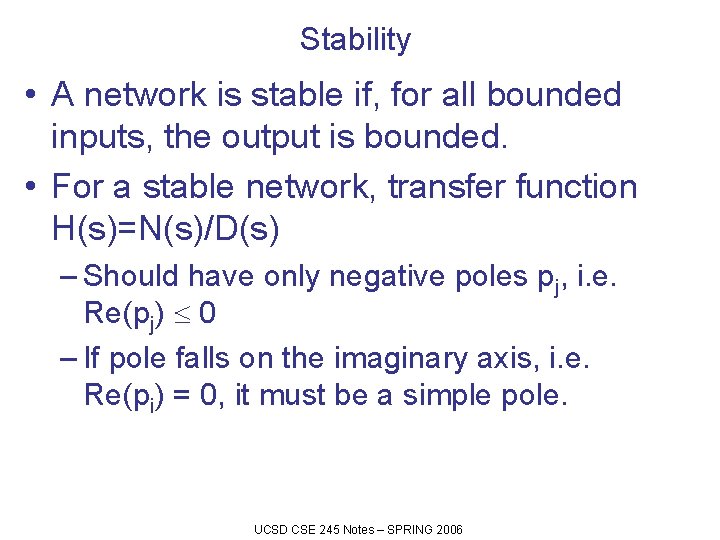
Stability • A network is stable if, for all bounded inputs, the output is bounded. • For a stable network, transfer function H(s)=N(s)/D(s) – Should have only negative poles pj, i. e. Re(pj) 0 – If pole falls on the imaginary axis, i. e. Re(pi) = 0, it must be a simple pole. UCSD CSE 245 Notes – SPRING 2006

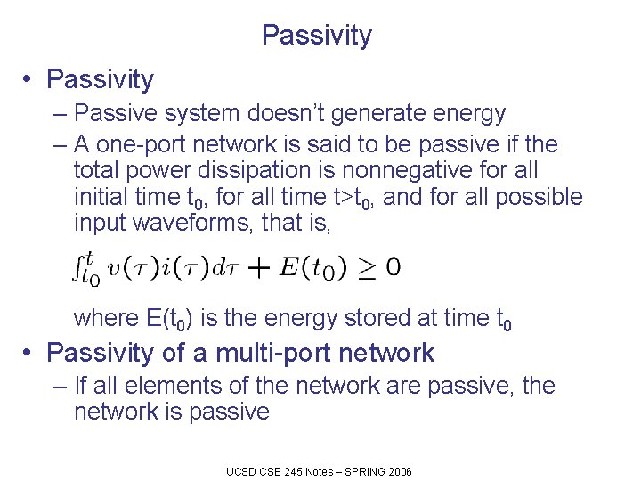
Passivity • Passivity – Passive system doesn’t generate energy – A one-port network is said to be passive if the total power dissipation is nonnegative for all initial time t 0, for all time t>t 0, and for all possible input waveforms, that is, where E(t 0) is the energy stored at time t 0 • Passivity of a multi-port network – If all elements of the network are passive, the network is passive UCSD CSE 245 Notes – SPRING 2006

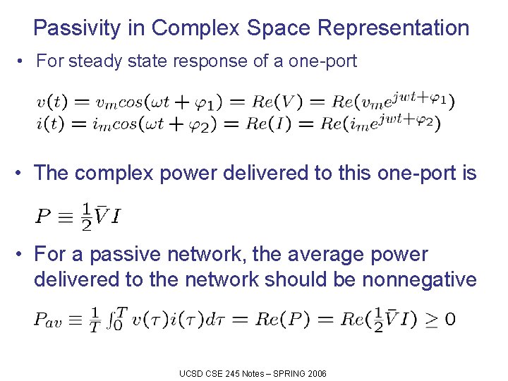
Passivity in Complex Space Representation • For steady state response of a one-port • The complex power delivered to this one-port is • For a passive network, the average power delivered to the network should be nonnegative UCSD CSE 245 Notes – SPRING 2006

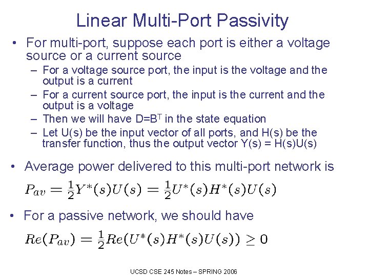
Linear Multi-Port Passivity • For multi-port, suppose each port is either a voltage source or a current source – For a voltage source port, the input is the voltage and the output is a current – For a current source port, the input is the current and the output is a voltage – Then we will have D=BT in the state equation – Let U(s) be the input vector of all ports, and H(s) be the transfer function, thus the output vector Y(s) = H(s)U(s) • Average power delivered to this multi-port network is • For a passive network, we should have UCSD CSE 245 Notes – SPRING 2006

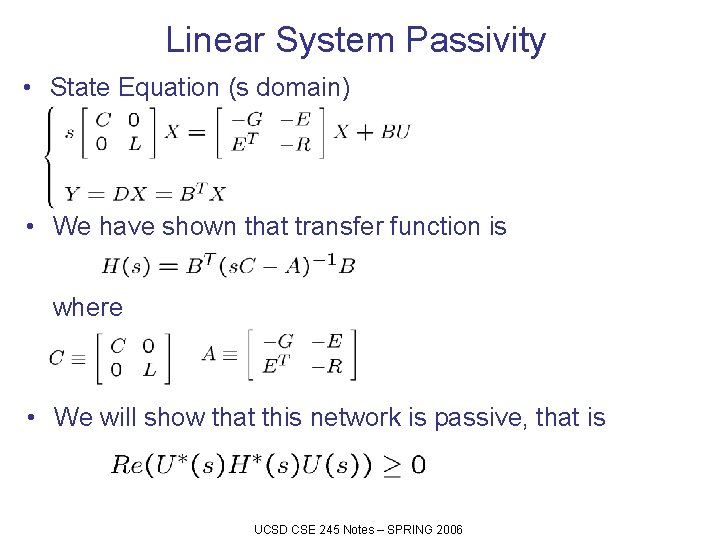
Linear System Passivity • State Equation (s domain) • We have shown that transfer function is where • We will show that this network is passive, that is UCSD CSE 245 Notes – SPRING 2006

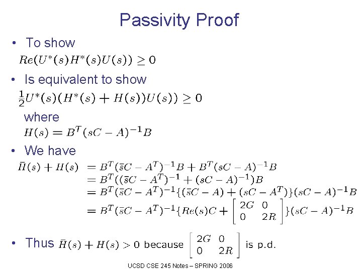
Passivity Proof • To show • Is equivalent to show where • We have • Thus UCSD CSE 245 Notes – SPRING 2006

Passivity and Stability • A passive network is stable. • However, a stable network is not necessarily passive. • The interconnection of passive models is a passive model • However, the interconnection of stable models is not necessarily stable UCSD CSE 245 Notes – SPRING 2006

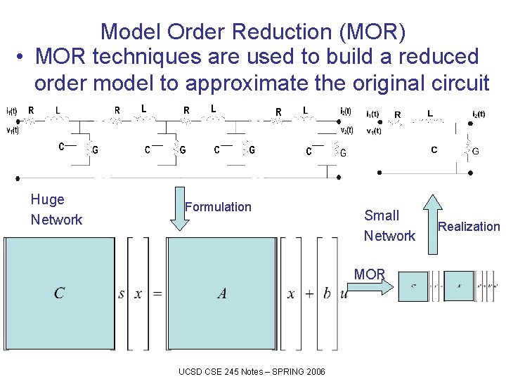
Model Order Reduction (MOR) • MOR techniques are used to build a reduced order model to approximate the original circuit Huge Network Formulation Small Network MOR UCSD CSE 245 Notes – SPRING 2006 Realization

Model Order Reduction: Overview • Explicit Moment Matching – AWE, Pade Approximation • Implicit Moment Matching – Krylov Subspace Methods • PRIMA, SPRIM • Gaussian Elimination – TICER – Y-Delta Transformation UCSD CSE 245 Notes – SPRING 2006

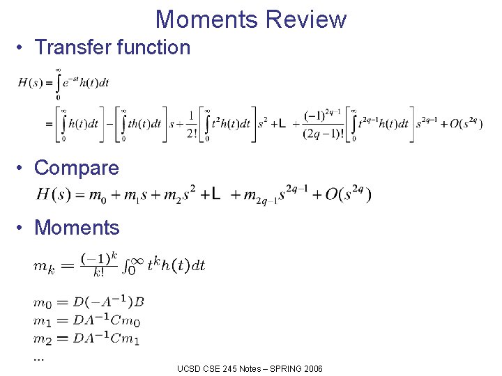
Moments Review • Transfer function • Compare • Moments UCSD CSE 245 Notes – SPRING 2006

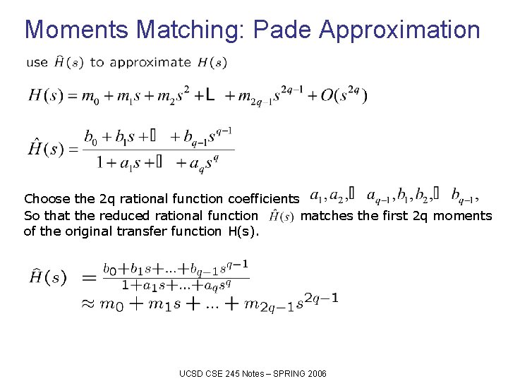
Moments Matching: Pade Approximation Choose the 2 q rational function coefficients So that the reduced rational function matches the first 2 q moments of the original transfer function H(s). UCSD CSE 245 Notes – SPRING 2006

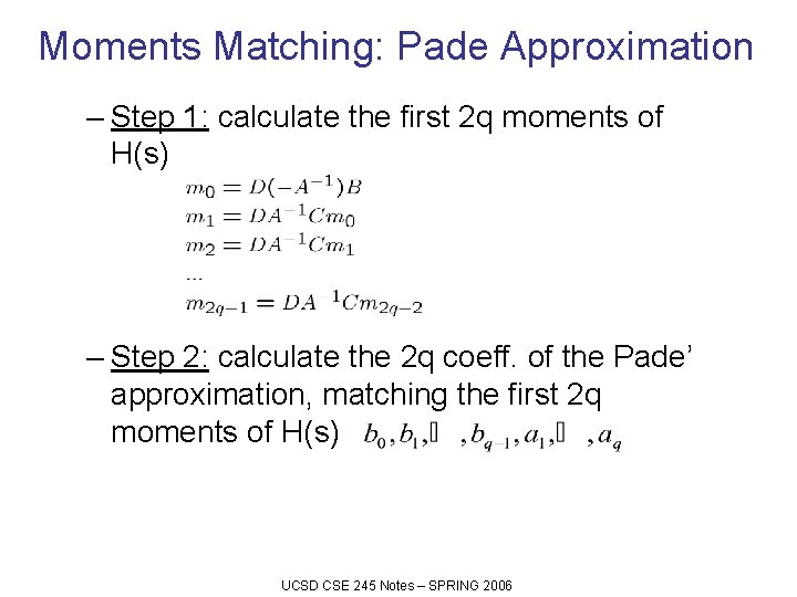
Moments Matching: Pade Approximation – Step 1: calculate the first 2 q moments of H(s) – Step 2: calculate the 2 q coeff. of the Pade’ approximation, matching the first 2 q moments of H(s) UCSD CSE 245 Notes – SPRING 2006

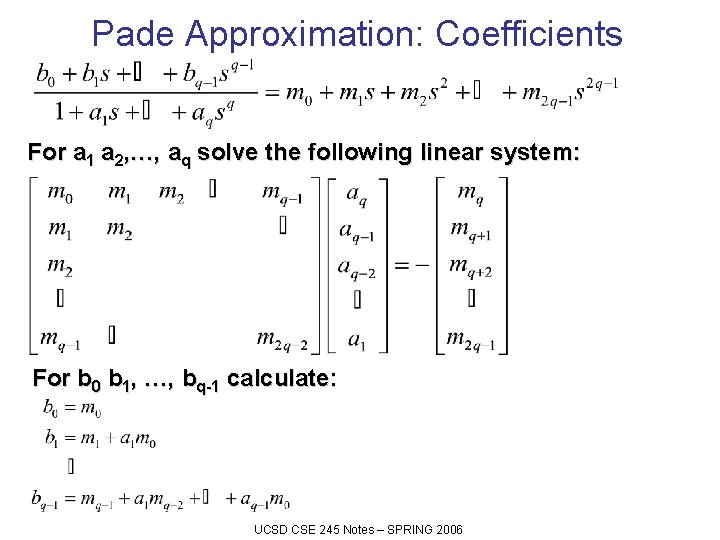
Pade Approximation: Coefficients For a 1 a 2, …, aq solve the following linear system: For b 0 b 1, …, bq-1 calculate: UCSD CSE 245 Notes – SPRING 2006

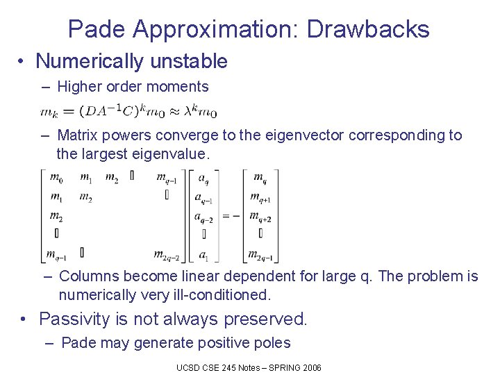
Pade Approximation: Drawbacks • Numerically unstable – Higher order moments – Matrix powers converge to the eigenvector corresponding to the largest eigenvalue. – Columns become linear dependent for large q. The problem is numerically very ill-conditioned. • Passivity is not always preserved. – Pade may generate positive poles UCSD CSE 245 Notes – SPRING 2006