Credit Risk Chapter 22 Options Futures and Other

Credit Risk Chapter 22 Options, Futures, and Other Derivatives, 7 th Edition, Copyright © John C. Hull 2008 1

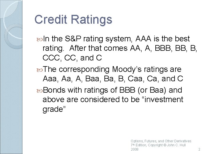
Credit Ratings In the S&P rating system, AAA is the best rating. After that comes AA, A, BBB, B, CCC, and C The corresponding Moody’s ratings are Aaa, A, Baa, B, Caa, Ca, and C Bonds with ratings of BBB (or Baa) and above are considered to be “investment grade” Options, Futures, and Other Derivatives 7 th Edition, Copyright © John C. Hull 2008 2

Historical Data Historical data provided by rating agencies are also used to estimate the probability of default Options, Futures, and Other Derivatives 7 th Edition, Copyright © John C. Hull 2008 3

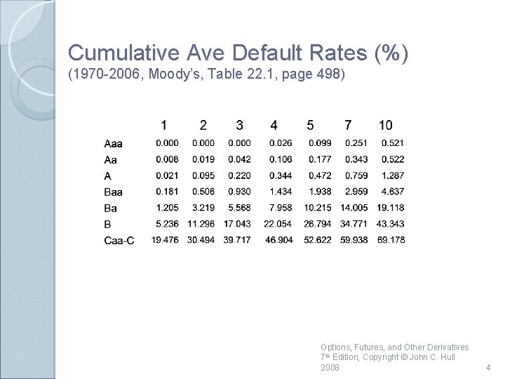
Cumulative Ave Default Rates (%) (1970 -2006, Moody’s, Table 22. 1, page 498) Options, Futures, and Other Derivatives 7 th Edition, Copyright © John C. Hull 2008 4

Interpretation The table shows the probability of default for companies starting with a particular credit rating A company with an initial credit rating of Baa has a probability of 0. 181% of defaulting by the end of the first year, 0. 506% by the end of the second year, and so on Options, Futures, and Other Derivatives 7 th Edition, Copyright © John C. Hull 2008 5

Do Default Probabilities Increase with Time? For a company that starts with a good credit rating default probabilities tend to increase with time For a company that starts with a poor credit rating default probabilities tend to decrease with time Options, Futures, and Other Derivatives 7 th Edition, Copyright © John C. Hull 2008 6

Default Intensities vs Unconditional Default Probabilities (page 498 -99) The default intensity (also called hazard rate) is the probability of default for a certain time period conditional on no earlier default The unconditional default probability is the probability of default for a certain time period as seen at time zero What are the default intensities and unconditional default probabilities for a Caa rate company in the third year? Options, Futures, and Other Derivatives 7 th Edition, Copyright © John C. Hull 2008 7

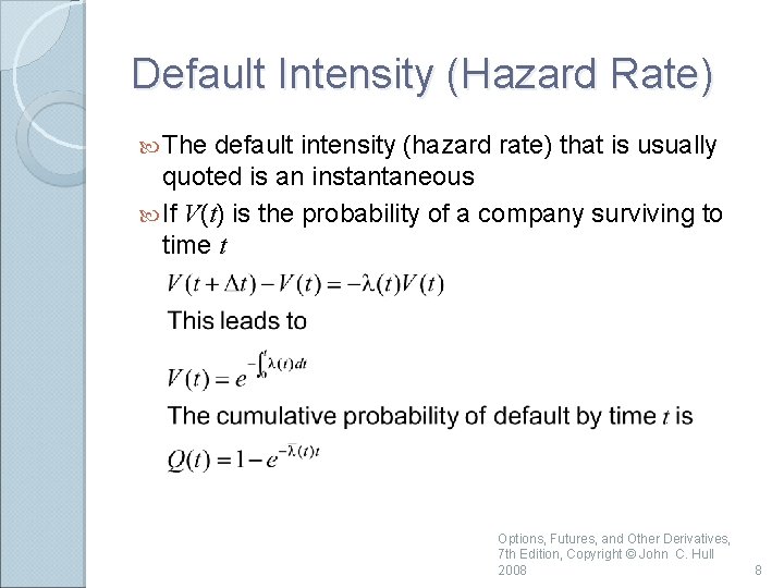
Default Intensity (Hazard Rate) The default intensity (hazard rate) that is usually quoted is an instantaneous If V(t) is the probability of a company surviving to time t Options, Futures, and Other Derivatives, 7 th Edition, Copyright © John C. Hull 2008 8

Recovery Rate The recovery rate for a bond is usually defined as the price of the bond immediately after default as a percent of its face value Options, Futures, and Other Derivatives 7 th Edition, Copyright © John C. Hull 2008 9

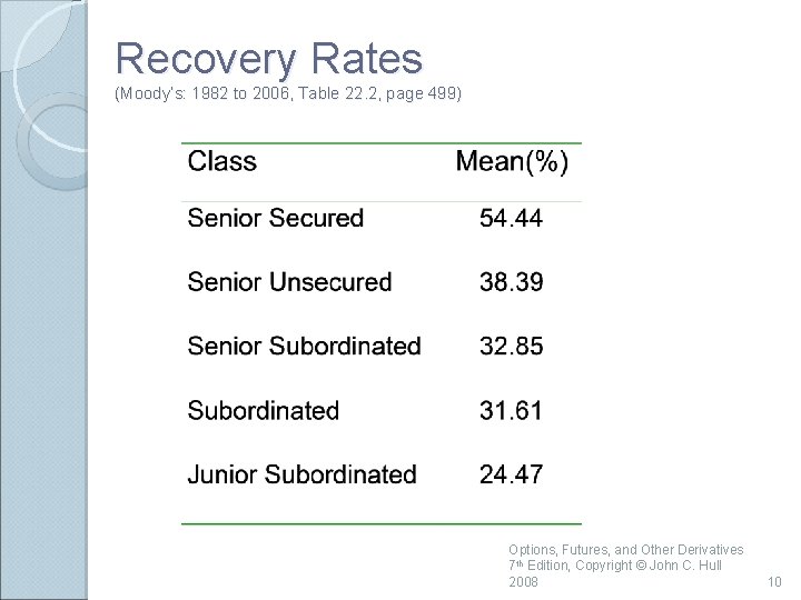
Recovery Rates (Moody’s: 1982 to 2006, Table 22. 2, page 499) Options, Futures, and Other Derivatives 7 th Edition, Copyright © John C. Hull 2008 10

Estimating Default Probabilities Alternatives: ◦ ◦ Use Bond Prices Use CDS spreads Use Historical Data Use Merton’s Model Options, Futures, and Other Derivatives 7 th Edition, Copyright © John C. Hull 2008 11

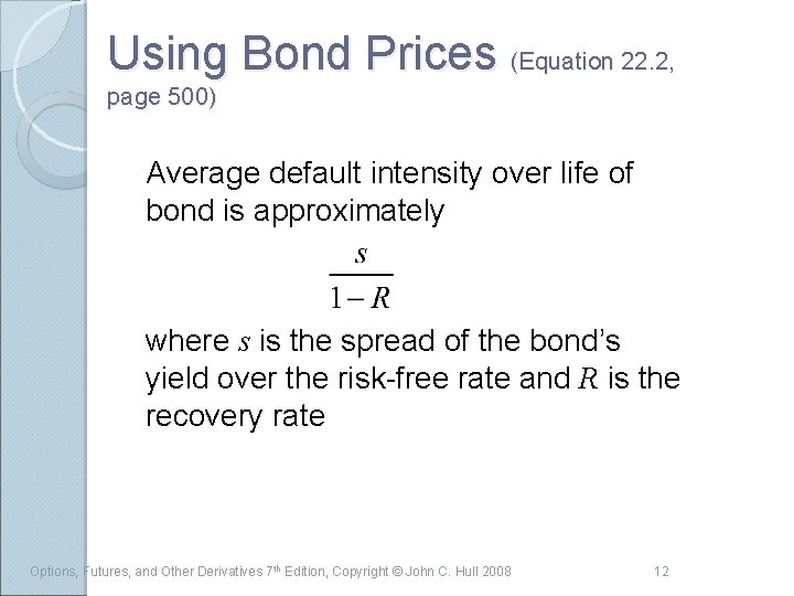
Using Bond Prices (Equation 22. 2, page 500) Average default intensity over life of bond is approximately where s is the spread of the bond’s yield over the risk-free rate and R is the recovery rate Options, Futures, and Other Derivatives 7 th Edition, Copyright © John C. Hull 2008 12

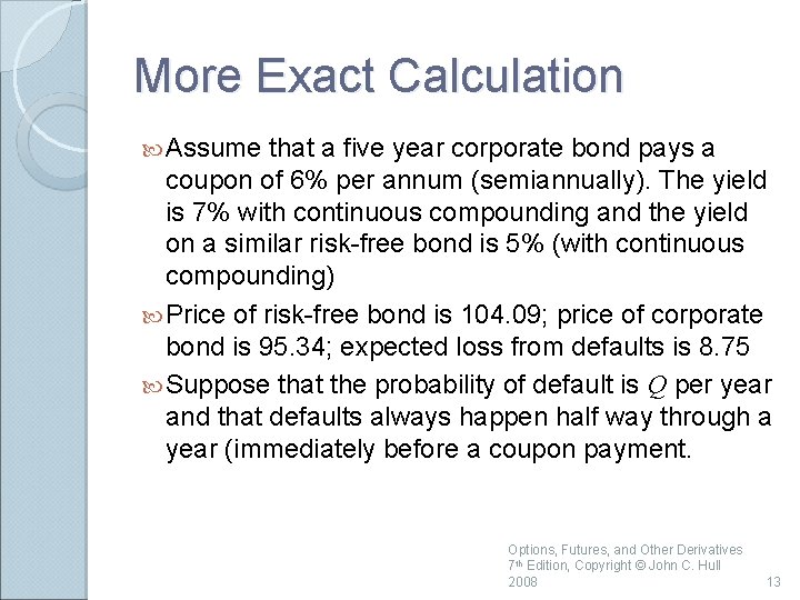
More Exact Calculation Assume that a five year corporate bond pays a coupon of 6% per annum (semiannually). The yield is 7% with continuous compounding and the yield on a similar risk-free bond is 5% (with continuous compounding) Price of risk-free bond is 104. 09; price of corporate bond is 95. 34; expected loss from defaults is 8. 75 Suppose that the probability of default is Q per year and that defaults always happen half way through a year (immediately before a coupon payment. Options, Futures, and Other Derivatives 7 th Edition, Copyright © John C. Hull 2008 13

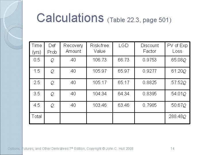
Calculations (Table 22. 3, page 501) Time (yrs) Def Prob Recovery Amount Risk-free Value LGD Discount Factor PV of Exp Loss 0. 5 Q 40 106. 73 66. 73 0. 9753 65. 08 Q 1. 5 Q 40 105. 97 65. 97 0. 9277 61. 20 Q 2. 5 Q 40 105. 17 65. 17 0. 8825 57. 52 Q 3. 5 Q 40 104. 34 64. 34 0. 8395 54. 01 Q 4. 5 Q 40 103. 46 63. 46 0. 7985 50. 67 Q Total Options, Futures, and Other Derivatives 7 th Edition, Copyright © John C. Hull 2008 288. 48 Q 14

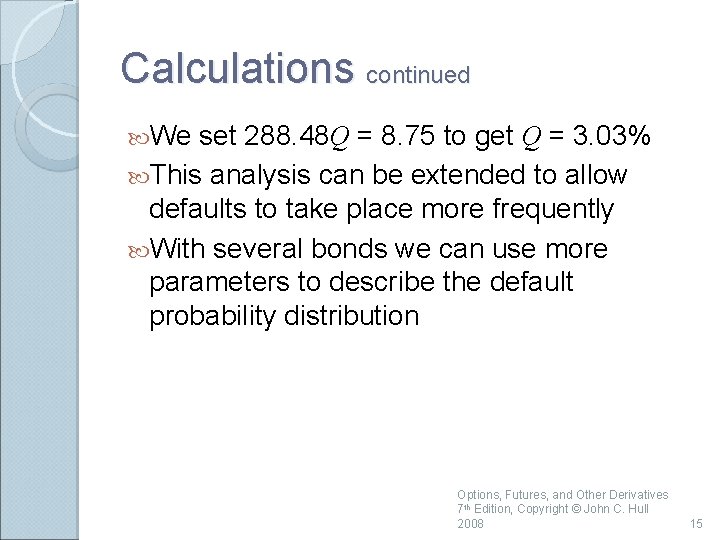
Calculations continued We set 288. 48 Q = 8. 75 to get Q = 3. 03% This analysis can be extended to allow defaults to take place more frequently With several bonds we can use more parameters to describe the default probability distribution Options, Futures, and Other Derivatives 7 th Edition, Copyright © John C. Hull 2008 15

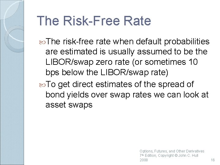
The Risk-Free Rate The risk-free rate when default probabilities are estimated is usually assumed to be the LIBOR/swap zero rate (or sometimes 10 bps below the LIBOR/swap rate) To get direct estimates of the spread of bond yields over swap rates we can look at asset swaps Options, Futures, and Other Derivatives 7 th Edition, Copyright © John C. Hull 2008 16

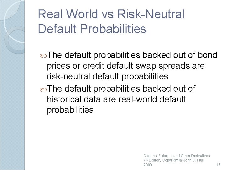
Real World vs Risk-Neutral Default Probabilities The default probabilities backed out of bond prices or credit default swap spreads are risk-neutral default probabilities The default probabilities backed out of historical data are real-world default probabilities Options, Futures, and Other Derivatives 7 th Edition, Copyright © John C. Hull 2008 17

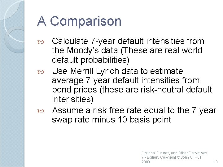
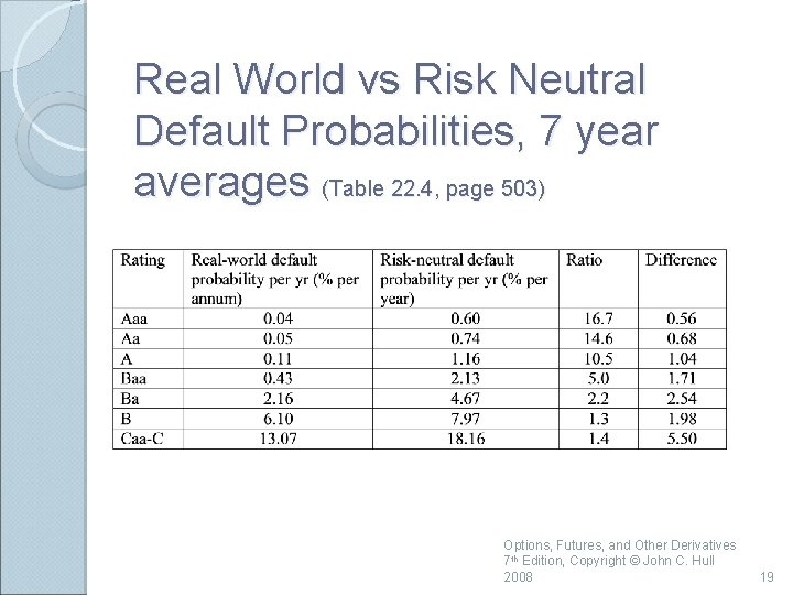
A Comparison Calculate 7 -year default intensities from the Moody’s data (These are real world default probabilities) Use Merrill Lynch data to estimate average 7 -year default intensities from bond prices (these are risk-neutral default intensities) Assume a risk-free rate equal to the 7 -year swap rate minus 10 basis point Options, Futures, and Other Derivatives 7 th Edition, Copyright © John C. Hull 2008 18

Real World vs Risk Neutral Default Probabilities, 7 year averages (Table 22. 4, page 503) Options, Futures, and Other Derivatives 7 th Edition, Copyright © John C. Hull 2008 19

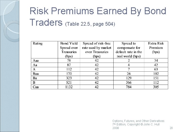
Risk Premiums Earned By Bond Traders (Table 22. 5, page 504) Options, Futures, and Other Derivatives 7 th Edition, Copyright © John C. Hull 2008 20

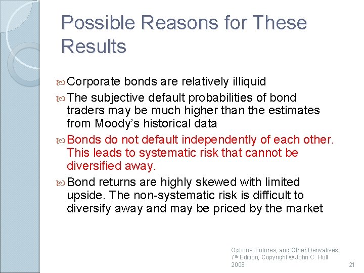
Possible Reasons for These Results Corporate bonds are relatively illiquid The subjective default probabilities of bond traders may be much higher than the estimates from Moody’s historical data Bonds do not default independently of each other. This leads to systematic risk that cannot be diversified away. Bond returns are highly skewed with limited upside. The non-systematic risk is difficult to diversify away and may be priced by the market Options, Futures, and Other Derivatives 7 th Edition, Copyright © John C. Hull 2008 21

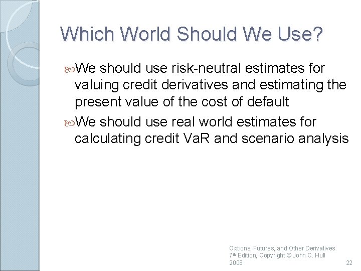
Which World Should We Use? We should use risk-neutral estimates for valuing credit derivatives and estimating the present value of the cost of default We should use real world estimates for calculating credit Va. R and scenario analysis Options, Futures, and Other Derivatives 7 th Edition, Copyright © John C. Hull 2008 22

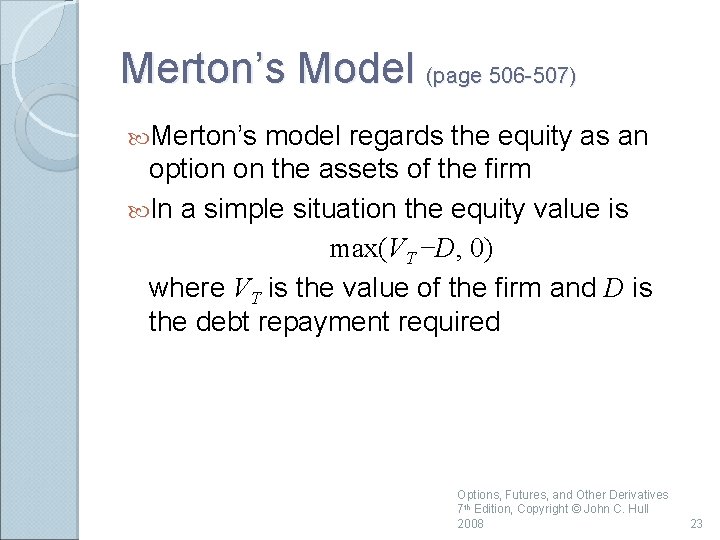
Merton’s Model (page 506 -507) Merton’s model regards the equity as an option on the assets of the firm In a simple situation the equity value is max(VT −D, 0) where VT is the value of the firm and D is the debt repayment required Options, Futures, and Other Derivatives 7 th Edition, Copyright © John C. Hull 2008 23

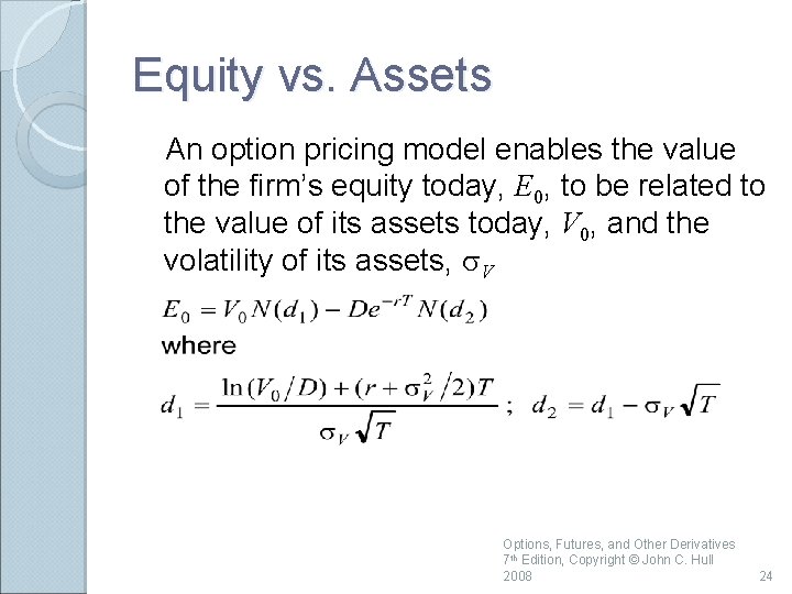
Equity vs. Assets An option pricing model enables the value of the firm’s equity today, E 0, to be related to the value of its assets today, V 0, and the volatility of its assets, s. V Options, Futures, and Other Derivatives 7 th Edition, Copyright © John C. Hull 2008 24

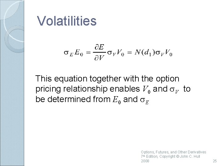
Volatilities This equation together with the option pricing relationship enables V 0 and s. V to be determined from E 0 and s. E Options, Futures, and Other Derivatives 7 th Edition, Copyright © John C. Hull 2008 25

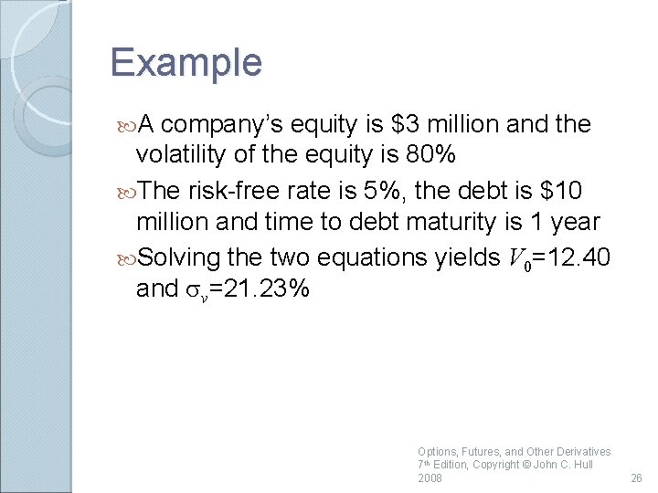
Example A company’s equity is $3 million and the volatility of the equity is 80% The risk-free rate is 5%, the debt is $10 million and time to debt maturity is 1 year Solving the two equations yields V 0=12. 40 and sv=21. 23% Options, Futures, and Other Derivatives 7 th Edition, Copyright © John C. Hull 2008 26

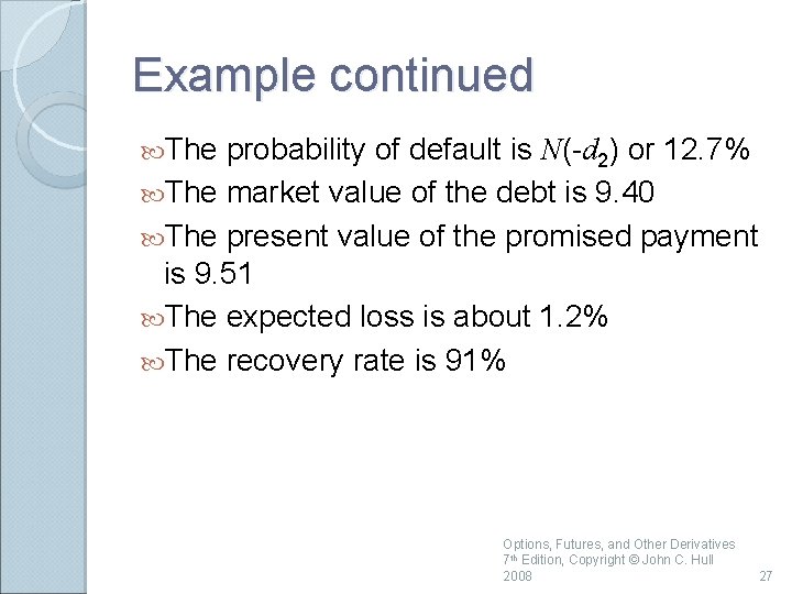
Example continued The probability of default is N(-d 2) or 12. 7% The market value of the debt is 9. 40 The present value of the promised payment is 9. 51 The expected loss is about 1. 2% The recovery rate is 91% Options, Futures, and Other Derivatives 7 th Edition, Copyright © John C. Hull 2008 27

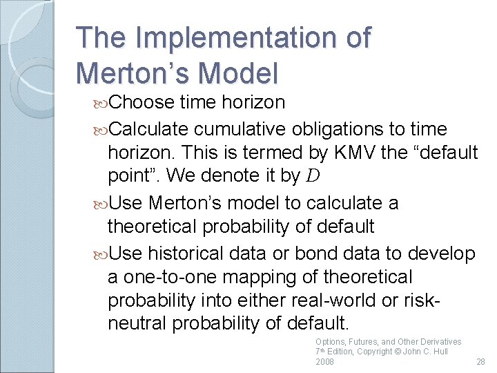
The Implementation of Merton’s Model Choose time horizon Calculate cumulative obligations to time horizon. This is termed by KMV the “default point”. We denote it by D Use Merton’s model to calculate a theoretical probability of default Use historical data or bond data to develop a one-to-one mapping of theoretical probability into either real-world or riskneutral probability of default. Options, Futures, and Other Derivatives 7 th Edition, Copyright © John C. Hull 2008 28

Credit Risk in Derivatives Transactions (page 510 -512) Three cases Contract always an asset Contract always a liability Contract can be an asset or a liability Options, Futures, and Other Derivatives 7 th Edition, Copyright © John C. Hull 2008 29

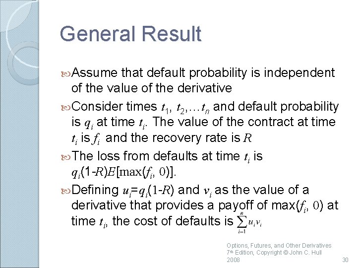
General Result Assume that default probability is independent of the value of the derivative Consider times t 1, t 2, …tn and default probability is qi at time ti. The value of the contract at time ti is fi and the recovery rate is R The loss from defaults at time ti is qi(1 -R)E[max(fi, 0)]. Defining ui=qi(1 -R) and vi as the value of a derivative that provides a payoff of max(fi, 0) at time ti, the cost of defaults is Options, Futures, and Other Derivatives 7 th Edition, Copyright © John C. Hull 2008 30

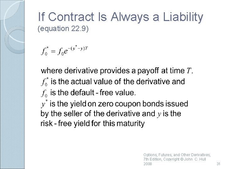
If Contract Is Always a Liability (equation 22. 9) Options, Futures, and Other Derivatives, 7 th Edition, Copyright © John C. Hull 2008 31

Credit Risk Mitigation Netting Collateralization Downgrade triggers Options, Futures, and Other Derivatives 7 th Edition, Copyright © John C. Hull 2008 32

Default Correlation The credit default correlation between two companies is a measure of their tendency to default at about the same time Default correlation is important in risk management when analyzing the benefits of credit risk diversification It is also important in the valuation of some credit derivatives, eg a first-to-default CDS and CDO tranches. Options, Futures, and Other Derivatives 7 th Edition, Copyright © John C. Hull 2008 33

Measurement There is no generally accepted measure of default correlation Default correlation is a more complex phenomenon than the correlation between two random variables Options, Futures, and Other Derivatives 7 th Edition, Copyright © John C. Hull 2008 34

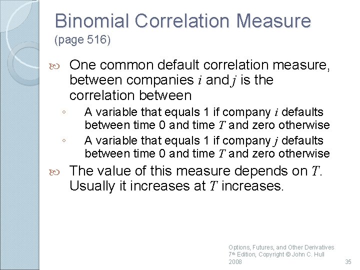
Binomial Correlation Measure (page 516) One common default correlation measure, between companies i and j is the correlation between ◦ ◦ A variable that equals 1 if company i defaults between time 0 and time T and zero otherwise A variable that equals 1 if company j defaults between time 0 and time T and zero otherwise The value of this measure depends on T. Usually it increases at T increases. Options, Futures, and Other Derivatives 7 th Edition, Copyright © John C. Hull 2008 35

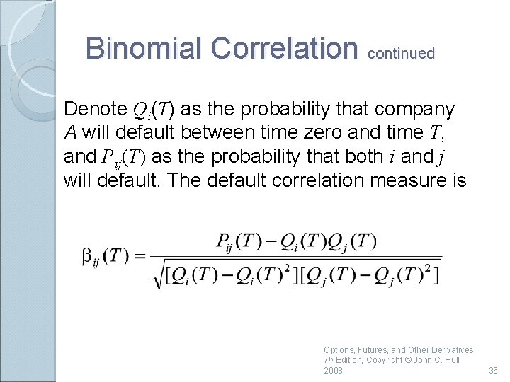
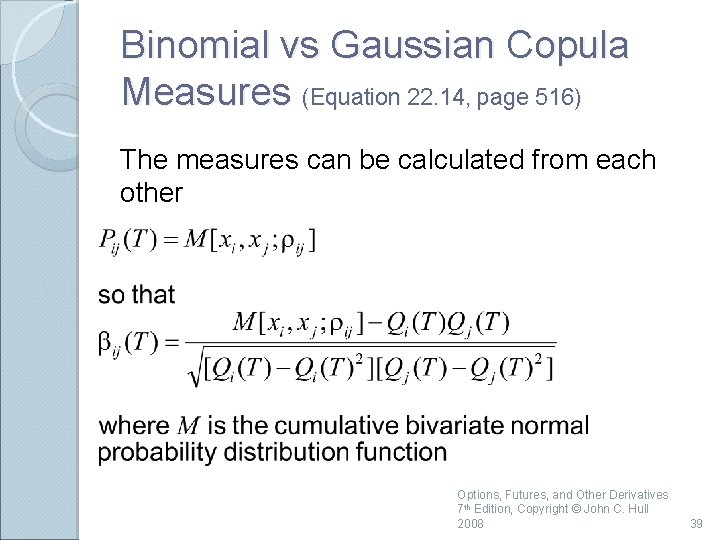
Binomial Correlation continued Denote Qi(T) as the probability that company A will default between time zero and time T, and Pij(T) as the probability that both i and j will default. The default correlation measure is Options, Futures, and Other Derivatives 7 th Edition, Copyright © John C. Hull 2008 36

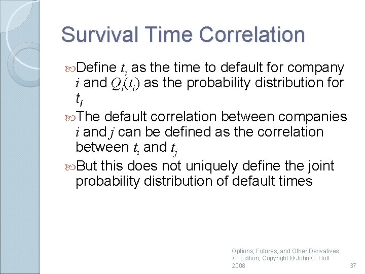
Survival Time Correlation Define ti as the time to default for company i and Qi(ti) as the probability distribution for ti The default correlation between companies i and j can be defined as the correlation between ti and tj But this does not uniquely define the joint probability distribution of default times Options, Futures, and Other Derivatives 7 th Edition, Copyright © John C. Hull 2008 37

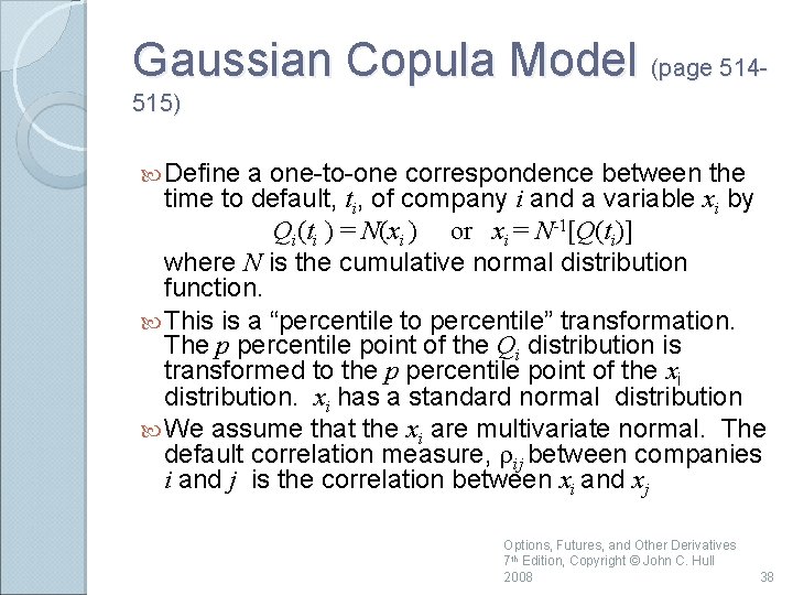
Gaussian Copula Model (page 514515) Define a one-to-one correspondence between the time to default, ti, of company i and a variable xi by Qi(ti ) = N(xi ) or xi = N-1[Q(ti)] where N is the cumulative normal distribution function. This is a “percentile to percentile” transformation. The p percentile point of the Qi distribution is transformed to the p percentile point of the xi distribution. xi has a standard normal distribution We assume that the xi are multivariate normal. The default correlation measure, rij between companies i and j is the correlation between xi and xj Options, Futures, and Other Derivatives 7 th Edition, Copyright © John C. Hull 2008 38

Binomial vs Gaussian Copula Measures (Equation 22. 14, page 516) The measures can be calculated from each other Options, Futures, and Other Derivatives 7 th Edition, Copyright © John C. Hull 2008 39

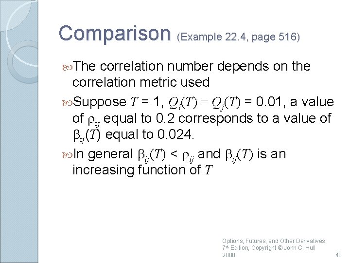
Comparison (Example 22. 4, page 516) The correlation number depends on the correlation metric used Suppose T = 1, Qi(T) = Qj(T) = 0. 01, a value of rij equal to 0. 2 corresponds to a value of bij(T) equal to 0. 024. In general bij(T) < rij and bij(T) is an increasing function of T Options, Futures, and Other Derivatives 7 th Edition, Copyright © John C. Hull 2008 40

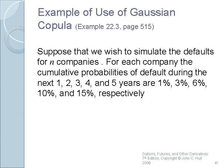
Example of Use of Gaussian Copula (Example 22. 3, page 515) Suppose that we wish to simulate the defaults for n companies. For each company the cumulative probabilities of default during the next 1, 2, 3, 4, and 5 years are 1%, 3%, 6%, 10%, and 15%, respectively Options, Futures, and Other Derivatives 7 th Edition, Copyright © John C. Hull 2008 41

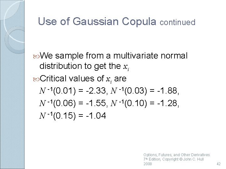
Use of Gaussian Copula continued We sample from a multivariate normal distribution to get the xi Critical values of xi are N -1(0. 01) = -2. 33, N -1(0. 03) = -1. 88, N -1(0. 06) = -1. 55, N -1(0. 10) = -1. 28, N -1(0. 15) = -1. 04 Options, Futures, and Other Derivatives 7 th Edition, Copyright © John C. Hull 2008 42

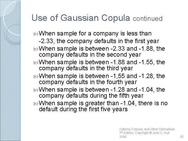
Use of Gaussian Copula continued When sample for a company is less than -2. 33, the company defaults in the first year When sample is between -2. 33 and -1. 88, the company defaults in the second year When sample is between -1. 88 and -1. 55, the company defaults in the third year When sample is between -1, 55 and -1. 28, the company defaults in the fourth year When sample is between -1. 28 and -1. 04, the company defaults during the fifth year When sample is greater than -1. 04, there is no default during the first five years Options, Futures, and Other Derivatives 7 th Edition, Copyright © John C. Hull 2008 43

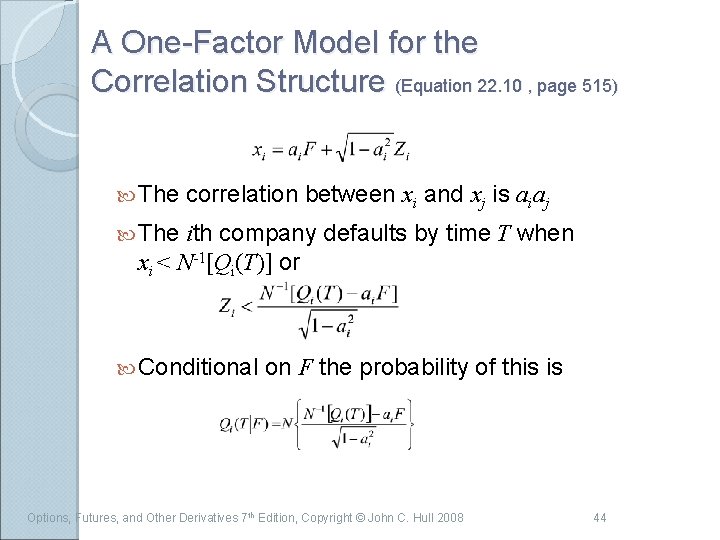
A One-Factor Model for the Correlation Structure (Equation 22. 10 , page 515) The correlation between xi and xj is aiaj The ith company defaults by time T when xi < N-1[Qi(T)] or Conditional on F the probability of this is Options, Futures, and Other Derivatives 7 th Edition, Copyright © John C. Hull 2008 44

Credit Va. R (page 517 -519) Can be defined analogously to Market Risk Va. R A T-year credit Va. R with an X% confidence is the loss level that we are X% confident will not be exceeded over T years Options, Futures, and Other Derivatives 7 th Edition, Copyright © John C. Hull 2008 45

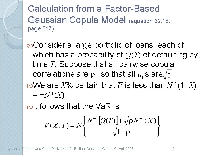
Calculation from a Factor-Based Gaussian Copula Model (equation 22. 15, page 517) Consider a large portfolio of loans, each of which has a probability of Q(T) of defaulting by time T. Suppose that all pairwise copula correlations are r so that all ai’s are We are X% certain that F is less than N-1(1−X) = −N-1(X) It follows that the Va. R is Options, Futures, and Other Derivatives 7 th Edition, Copyright © John C. Hull 2008 46

Basel II The internal ratings based approach uses the Gaussian copula model to calculate the 99. 9% worst case default rate for a portfolio This is multiplied by the loss given default (=1−Rec Rate), the expected exposure at default, and a maturity adjustment to give the capital required Options, Futures, and Other Derivatives, 7 th Edition, Copyright © John C. Hull 2008 47

Credit. Metrics (page 517 -519) Calculates credit Va. R by considering possible rating transitions A Gaussian copula model is used to define the correlation between the ratings transitions of different companies Options, Futures, and Other Derivatives 7 th Edition, Copyright © John C. Hull 2008 48