CPS 296 1 Learning in games Vincent Conitzer

CPS 296. 1 Learning in games Vincent Conitzer conitzer@cs. duke. edu

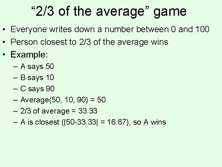
“ 2/3 of the average” game • Everyone writes down a number between 0 and 100 • Person closest to 2/3 of the average wins • Example: – – – A says 50 B says 10 C says 90 Average(50, 10, 90) = 50 2/3 of average = 33. 33 A is closest (|50 -33. 33| = 16. 67), so A wins

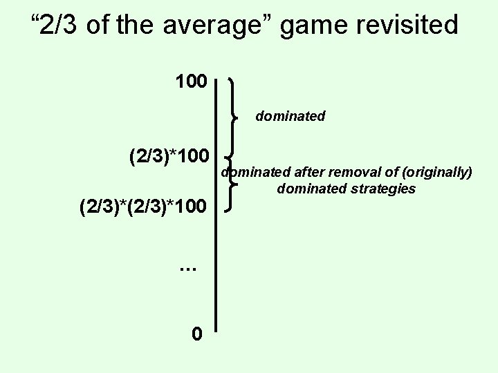
“ 2/3 of the average” game revisited 100 dominated (2/3)*100 … 0 dominated after removal of (originally) dominated strategies

Learning in (normal-form) games • Approach we have taken so far when playing a game: just compute an optimal/equilibrium strategy • Another approach: learn how to play a game by – playing it many times, and – updating your strategy based on experience • Why? – Some of the game’s utilities (especially the other players’) may be unknown to you – The other players may not be playing an equilibrium strategy – Computing an optimal strategy can be hard – Learning is what humans typically do – … • Learning strategies ~ strategies for the repeated game • Does learning converge to equilibrium?

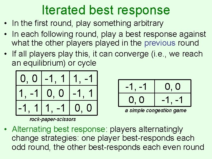
Iterated best response • In the first round, play something arbitrary • In each following round, play a best response against what the other players played in the previous round • If all players play this, it can converge (i. e. , we reach an equilibrium) or cycle 0, 0 -1, 1 1, -1 0, 0 -1, -1 a simple congestion game rock-paper-scissors • Alternating best response: players alternatingly change strategies: one player best-responds each odd round, the other best-responds each even round

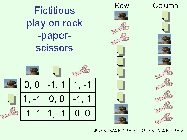
Fictitious play [Brown 1951] • In the first round, play something arbitrary • In each following round, play a best response against the empirical distribution of the other players’ play – I. e. , as if other player randomly selects from his past actions • Again, if this converges, we have a Nash equilibrium • Can still fail to converge… 0, 0 -1, 1 1, -1 0, 0 rock-paper-scissors -1, -1 0, 0 -1, -1 a simple congestion game

Fictitious play on rock -paperscissors Row Column 0, 0 -1, 1 1, -1 0, 0 30% R, 50% P, 20% S 30% R, 20% P, 50% S

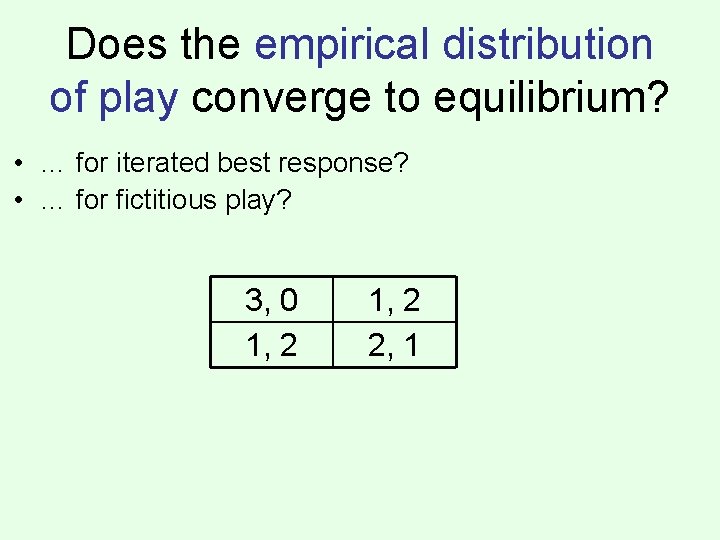
Does the empirical distribution of play converge to equilibrium? • … for iterated best response? • … for fictitious play? 3, 0 1, 2 2, 1

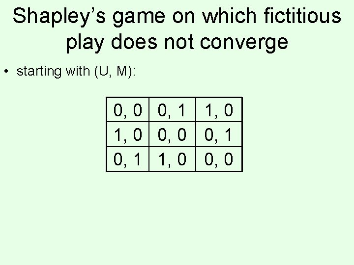
Fictitious play is guaranteed to converge in… • Two-player zero-sum games [Robinson 1951] • Generic 2 x 2 games [Miyasawa 1961] • Games solvable by iterated strict dominance [Nachbar 1990] • Weighted potential games [Monderer & Shapley 1996] • Not in general [Shapley 1964] • But, fictitious play always converges to the set of ½approximate equilibria [Conitzer 2009]

Shapley’s game on which fictitious play does not converge • starting with (U, M): 0, 0 0, 1 1, 0 0, 0

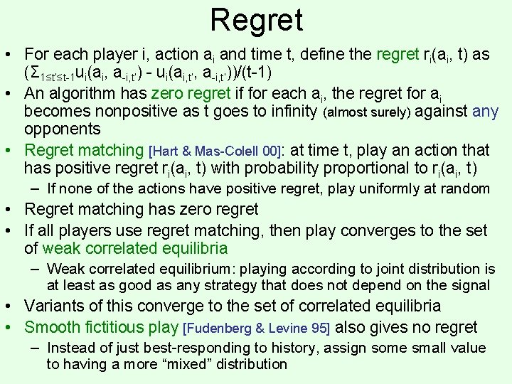
Regret • For each player i, action ai and time t, define the regret ri(ai, t) as (Σ 1≤t’≤t-1 ui(ai, a-i, t’) - ui(ai, t’, a-i, t’))/(t-1) • An algorithm has zero regret if for each ai, the regret for ai becomes nonpositive as t goes to infinity (almost surely) against any opponents • Regret matching [Hart & Mas-Colell 00]: at time t, play an action that has positive regret ri(ai, t) with probability proportional to ri(ai, t) – If none of the actions have positive regret, play uniformly at random • Regret matching has zero regret • If all players use regret matching, then play converges to the set of weak correlated equilibria – Weak correlated equilibrium: playing according to joint distribution is at least as good as any strategy that does not depend on the signal • Variants of this converge to the set of correlated equilibria • Smooth fictitious play [Fudenberg & Levine 95] also gives no regret – Instead of just best-responding to history, assign some small value to having a more “mixed” distribution

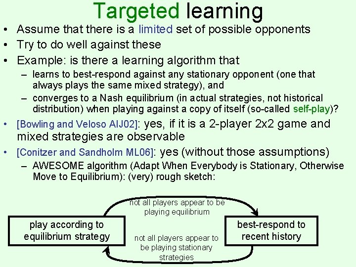
Targeted learning • Assume that there is a limited set of possible opponents • Try to do well against these • Example: is there a learning algorithm that – learns to best-respond against any stationary opponent (one that always plays the same mixed strategy), and – converges to a Nash equilibrium (in actual strategies, not historical distribution) when playing against a copy of itself (so-called self-play)? • [Bowling and Veloso AIJ 02]: yes, if it is a 2 -player 2 x 2 game and mixed strategies are observable • [Conitzer and Sandholm ML 06]: yes (without those assumptions) – AWESOME algorithm (Adapt When Everybody is Stationary, Otherwise Move to Equilibrium): (very) rough sketch: not all players appear to be playing equilibrium play according to equilibrium strategy not all players appear to be playing stationary strategies best-respond to recent history

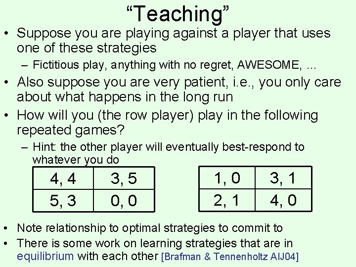
“Teaching” • Suppose you are playing against a player that uses one of these strategies – Fictitious play, anything with no regret, AWESOME, … • Also suppose you are very patient, i. e. , you only care about what happens in the long run • How will you (the row player) play in the following repeated games? – Hint: the other player will eventually best-respond to whatever you do 4, 4 5, 3 3, 5 0, 0 1, 0 2, 1 3, 1 4, 0 • Note relationship to optimal strategies to commit to • There is some work on learning strategies that are in equilibrium with each other [Brafman & Tennenholtz AIJ 04]

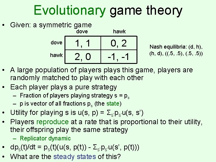
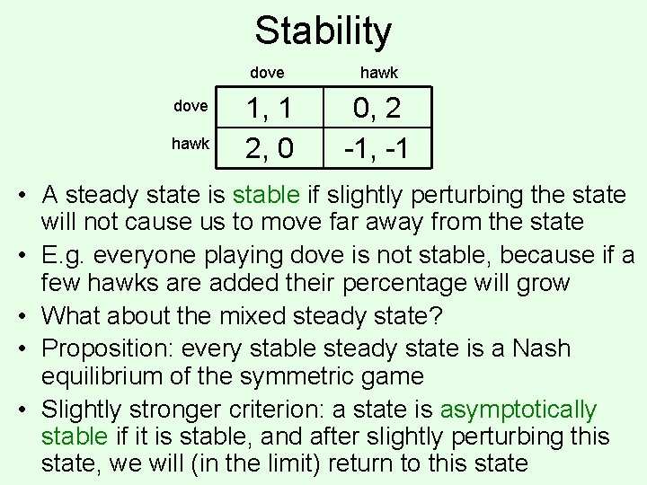
Evolutionary game theory • Given: a symmetric game dove hawk 1, 1 2, 0 0, 2 -1, -1 Nash equilibria: (d, h), (h, d), ((. 5, . 5), (. 5, . 5)) • A large population of players plays this game, players are randomly matched to play with each other • Each player plays a pure strategy – Fraction of players playing strategy s = ps – p is vector of all fractions ps (the state) • Utility for playing s is u(s, p) = Σs’ps’u(s, s’) • Players reproduce at a rate that is proportional to their utility, their offspring play the same strategy – Replicator dynamic • dps(t)/dt = ps(t)(u(s, p(t)) - Σs’ps’u(s’, p(t))) • What are the steady states of this?

Stability dove hawk 1, 1 2, 0 0, 2 -1, -1 • A steady state is stable if slightly perturbing the state will not cause us to move far away from the state • E. g. everyone playing dove is not stable, because if a few hawks are added their percentage will grow • What about the mixed steady state? • Proposition: every stable steady state is a Nash equilibrium of the symmetric game • Slightly stronger criterion: a state is asymptotically stable if it is stable, and after slightly perturbing this state, we will (in the limit) return to this state

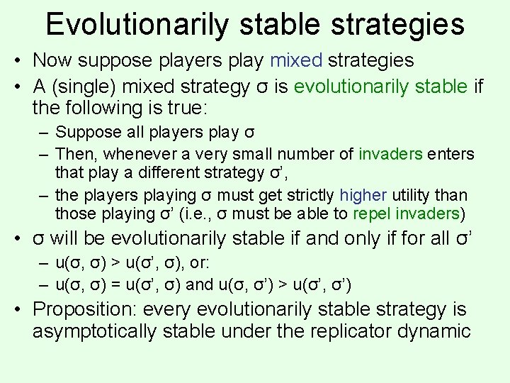
Evolutionarily stable strategies • Now suppose players play mixed strategies • A (single) mixed strategy σ is evolutionarily stable if the following is true: – Suppose all players play σ – Then, whenever a very small number of invaders enters that play a different strategy σ’, – the players playing σ must get strictly higher utility than those playing σ’ (i. e. , σ must be able to repel invaders) • σ will be evolutionarily stable if and only if for all σ’ – u(σ, σ) > u(σ’, σ), or: – u(σ, σ) = u(σ’, σ) and u(σ, σ’) > u(σ’, σ’) • Proposition: every evolutionarily stable strategy is asymptotically stable under the replicator dynamic