Constraint Satisfaction and Scheduling Andrew W Moore Professor

Constraint Satisfaction and Scheduling Andrew W. Moore Professor School of Computer Science Carnegie Mellon University www. cs. cmu. edu/~awm awm@cs. cmu. edu 412 -268 -7599 Note to other teachers and users of these slides. Andrew would be delighted if you found this source material useful in giving your own lectures. Feel free to use these slides verbatim, or to modify them to fit your own needs. Power. Point originals are available. If you make use of a significant portion of these slides in your own lecture, please include this message, or the following link to the source repository of Andrew’s tutorials: http: //www. cs. cmu. edu/~awm/tutorials. Comments and corrections gratefully received.

Overview • CSPs defined • Using standard search for CSPs • Blindingly obvious improvements § Backtracking search § Forward Checking § Constraint Propagation • Some example CSP applications § Overview § Waltz Algorithm § Job Shop Scheduling • Variable ordering • Value ordering • Tedious Discussion

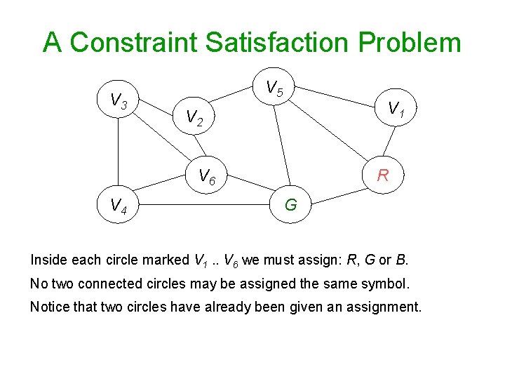
A Constraint Satisfaction Problem V 3 V 5 V 1 V 2 V 6 V 4 R G Inside each circle marked V 1. . V 6 we must assign: R, G or B. No two connected circles may be assigned the same symbol. Notice that two circles have already been given an assignment.

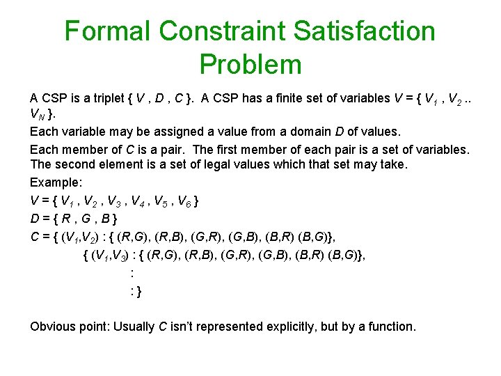
Formal Constraint Satisfaction Problem A CSP is a triplet { V , D , C }. A CSP has a finite set of variables V = { V 1 , V 2. . VN }. Each variable may be assigned a value from a domain D of values. Each member of C is a pair. The first member of each pair is a set of variables. The second element is a set of legal values which that set may take. Example: V = { V 1 , V 2 , V 3 , V 4 , V 5 , V 6 } D={R, G, B} C = { (V 1, V 2) : { (R, G), (R, B), (G, R), (G, B), (B, R) (B, G)}, { (V 1, V 3) : { (R, G), (R, B), (G, R), (G, B), (B, R) (B, G)}, : : } Obvious point: Usually C isn’t represented explicitly, but by a function.

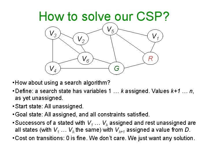
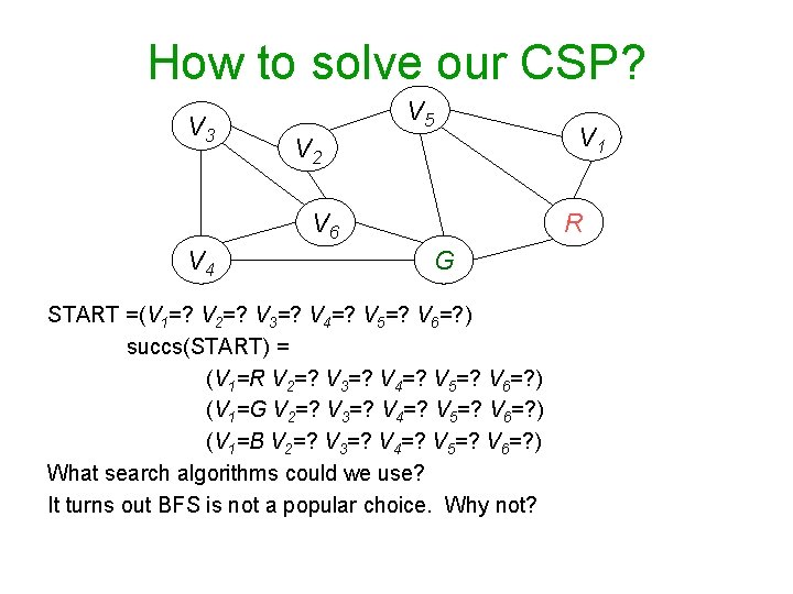
How to solve our CSP? V 3 V 5 V 2 V 6 V 4 V 1 R G • How about using a search algorithm? • Define: a search state has variables 1 … k assigned. Values k+1 … n, as yet unassigned. • Start state: All unassigned. • Goal state: All assigned, and all constraints satisfied. • Successors of a stated with V 1 … Vk assigned and rest unassigned are all states (with V 1 … Vk the same) with Vk+1 assigned a value from D. • Cost on transitions: 0 is fine. We don’t care. We just want any solution.

How to solve our CSP? V 3 V 5 V 2 V 6 V 4 V 1 R G START =(V 1=? V 2=? V 3=? V 4=? V 5=? V 6=? ) succs(START) = (V 1=R V 2=? V 3=? V 4=? V 5=? V 6=? ) (V 1=G V 2=? V 3=? V 4=? V 5=? V 6=? ) (V 1=B V 2=? V 3=? V 4=? V 5=? V 6=? ) What search algorithms could we use? It turns out BFS is not a popular choice. Why not?

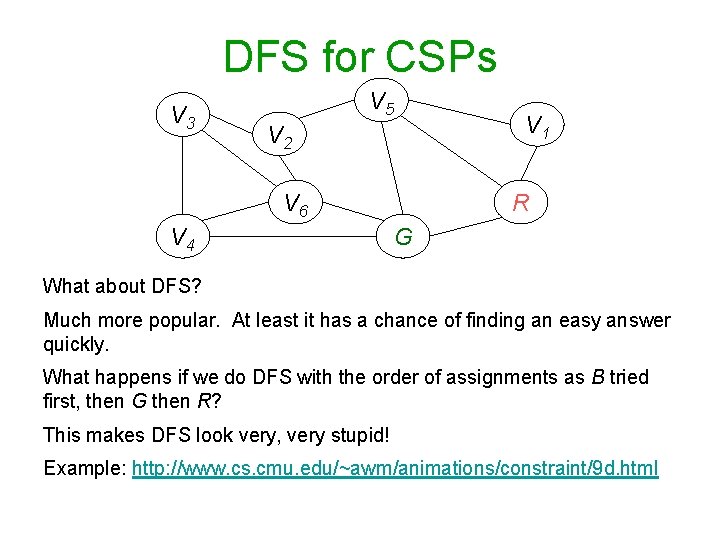
DFS for CSPs V 3 V 5 V 2 V 6 V 4 V 1 R G What about DFS? Much more popular. At least it has a chance of finding an easy answer quickly. What happens if we do DFS with the order of assignments as B tried first, then G then R? This makes DFS look very, very stupid! Example: http: //www. cs. cmu. edu/~awm/animations/constraint/9 d. html

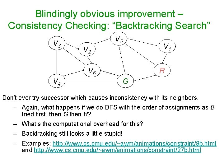
Blindingly obvious improvement – Consistency Checking: “Backtracking Search” V 3 V 5 V 2 V 6 V 4 V 1 R G Don’t ever try successor which causes inconsistency with its neighbors. – Again, what happens if we do DFS with the order of assignments as B tried first, then G then R? – What’s the computational overhead for this? – Backtracking still looks a little stupid! – Examples: http: //www. cs. cmu. edu/~awm/animations/constraint/9 b. html and http: //www. cs. cmu. edu/~awm/animations/constraint/27 b. html

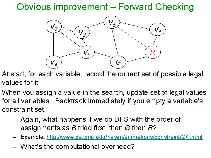
Obvious improvement – Forward Checking V 3 V 5 V 2 V 6 V 4 V 1 R G At start, for each variable, record the current set of possible legal values for it. When you assign a value in the search, update set of legal values for all variables. Backtrack immediately if you empty a variable’s constraint set. – Again, what happens if we do DFS with the order of assignments as B tried first, then G then R? – Example: http: //www. cs. cmu. edu/~awm/animations/constraint/27 f. html – What’s the computational overhead?

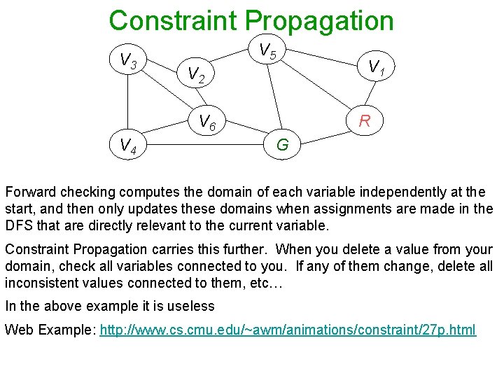
Constraint Propagation V 3 V 5 V 2 V 6 V 4 V 1 R G Forward checking computes the domain of each variable independently at the start, and then only updates these domains when assignments are made in the DFS that are directly relevant to the current variable. Constraint Propagation carries this further. When you delete a value from your domain, check all variables connected to you. If any of them change, delete all inconsistent values connected to them, etc… In the above example it is useless Web Example: http: //www. cs. cmu. edu/~awm/animations/constraint/27 p. html

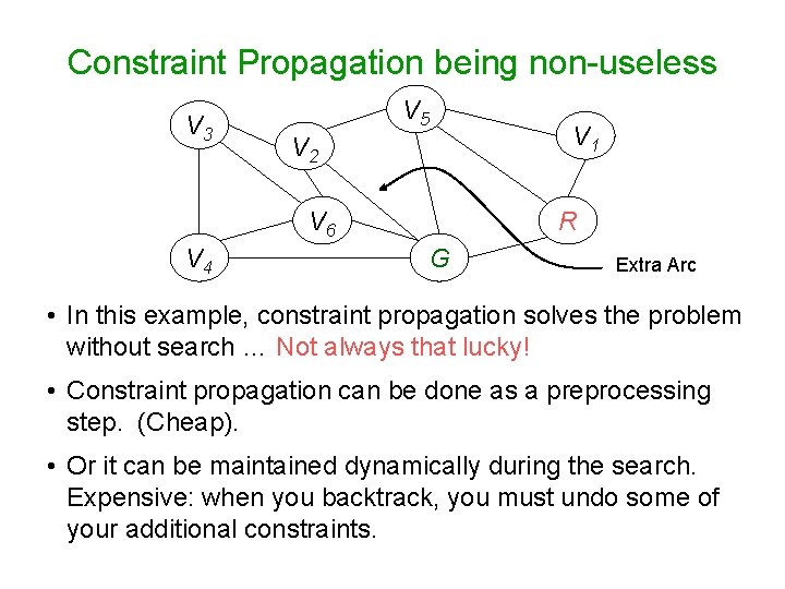
Constraint Propagation being non-useless V 3 V 5 V 2 V 6 V 4 V 1 R G Extra Arc • In this example, constraint propagation solves the problem without search … Not always that lucky! • Constraint propagation can be done as a preprocessing step. (Cheap). • Or it can be maintained dynamically during the search. Expensive: when you backtrack, you must undo some of your additional constraints.

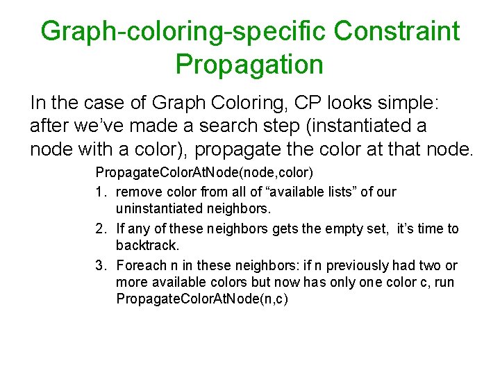
Graph-coloring-specific Constraint Propagation In the case of Graph Coloring, CP looks simple: after we’ve made a search step (instantiated a node with a color), propagate the color at that node. Propagate. Color. At. Node(node, color) 1. remove color from all of “available lists” of our uninstantiated neighbors. 2. If any of these neighbors gets the empty set, it’s time to backtrack. 3. Foreach n in these neighbors: if n previously had two or more available colors but now has only one color c, run Propagate. Color. At. Node(n, c)

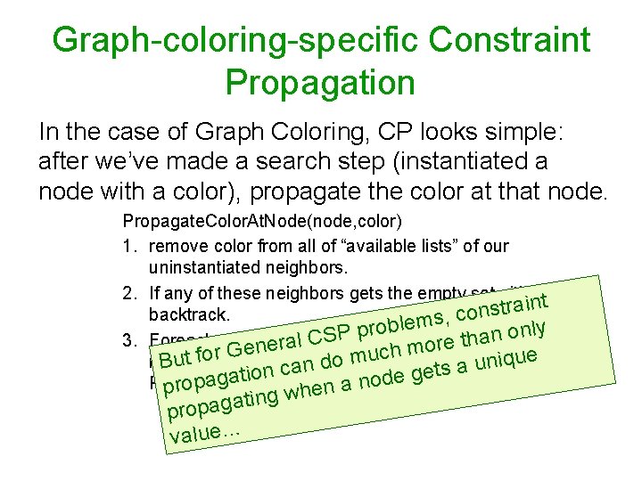
Graph-coloring-specific Constraint Propagation In the case of Graph Coloring, CP looks simple: after we’ve made a search step (instantiated a node with a color), propagate the color at that node. Propagate. Color. At. Node(node, color) 1. remove color from all of “available lists” of our uninstantiated neighbors. 2. If any of these neighbors gets the empty set, it’s time to t n i a str n o backtrack. c , s lem b o r p nlytwo or o P n S a C h 3. Foreach n inethese neighbors: if n previously had l t a ore ner m G h c r u o f ue c, run m q i o more but now has only one color But availablencolors n d u n a a c ts e o g i t e a d g o a Propagate. Color. At. Node(n, c) prop en a n h w g n i t a propag value…

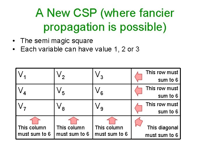
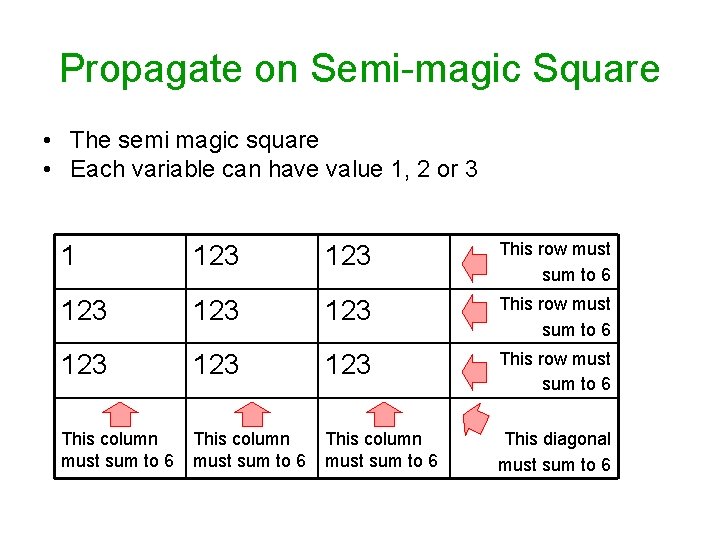
A New CSP (where fancier propagation is possible) • The semi magic square • Each variable can have value 1, 2 or 3 V 1 V 2 V 3 This row must sum to 6 V 4 V 5 V 6 This row must sum to 6 V 7 V 8 V 9 This row must sum to 6 This column must sum to 6 This diagonal must sum to 6

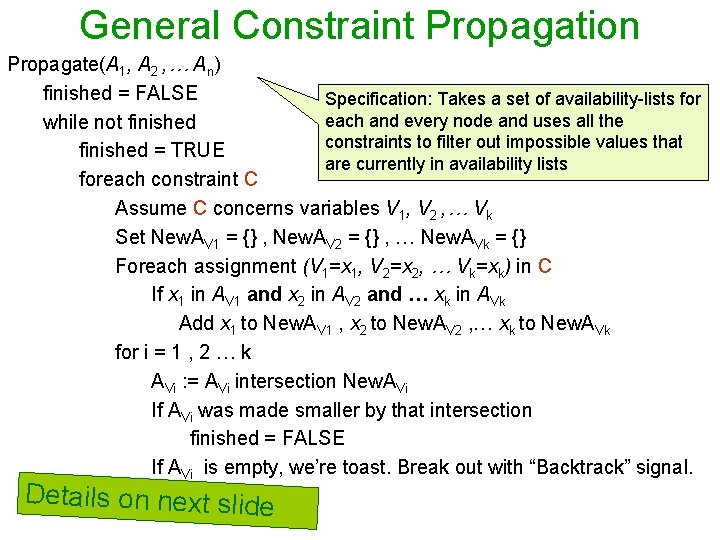
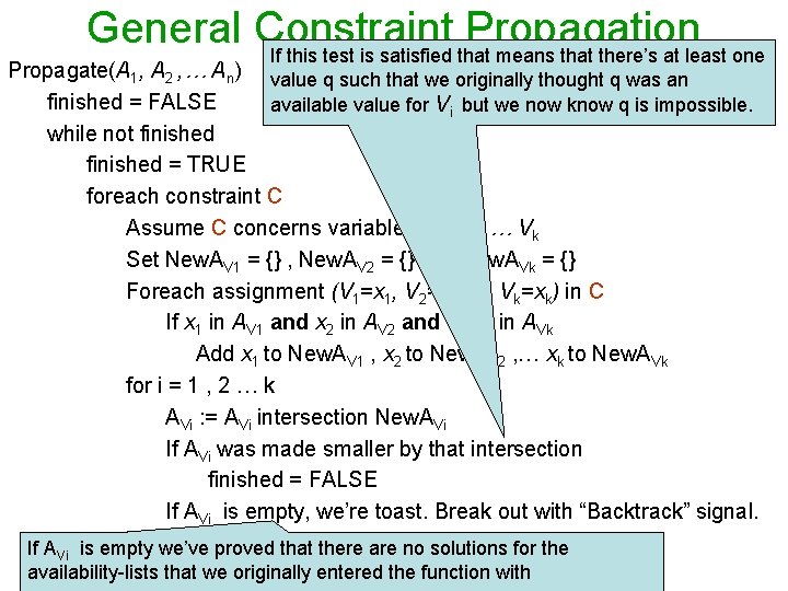
General Constraint Propagation Propagate(A 1, A 2 , … An) finished = FALSE Specification: Takes a set of availability-lists for each and every node and uses all the while not finished constraints to filter out impossible values that finished = TRUE are currently in availability lists foreach constraint C Assume C concerns variables V 1, V 2 , … Vk Set New. AV 1 = {} , New. AV 2 = {} , … New. AVk = {} Foreach assignment (V 1=x 1, V 2=x 2, … Vk=xk) in C If x 1 in AV 1 and x 2 in AV 2 and … xk in AVk Add x 1 to New. AV 1 , x 2 to New. AV 2 , … xk to New. AVk for i = 1 , 2 … k AVi : = AVi intersection New. AVi If AVi was made smaller by that intersection finished = FALSE If AVi is empty, we’re toast. Break out with “Backtrack” signal. Details on next slide

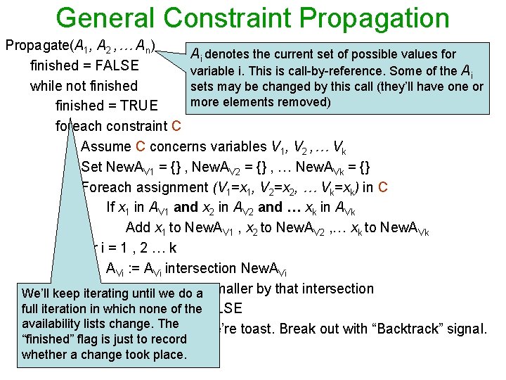
General Constraint Propagation Propagate(A 1, A 2 , … An) Ai denotes the current set of possible values for finished = FALSE variable i. This is call-by-reference. Some of the Ai while not finished sets may be changed by this call (they’ll have one or more elements removed) finished = TRUE foreach constraint C Assume C concerns variables V 1, V 2 , … Vk Set New. AV 1 = {} , New. AV 2 = {} , … New. AVk = {} Foreach assignment (V 1=x 1, V 2=x 2, … Vk=xk) in C If x 1 in AV 1 and x 2 in AV 2 and … xk in AVk Add x 1 to New. AV 1 , x 2 to New. AV 2 , … xk to New. AVk for i = 1 , 2 … k AVi : = AVi intersection New. AVi If AViuntil waswemade We’ll keep iterating do a smaller by that intersection full iteration in whichfinished none of the = FALSE availability lists Ifchange. The AVi is empty, we’re toast. Break out with “Backtrack” signal. “finished” flag is just to record whether a change took place.

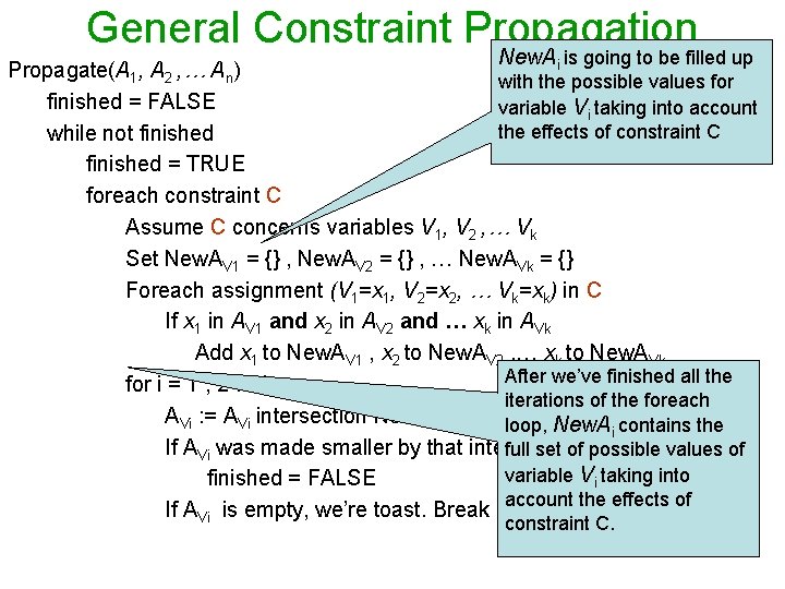
General Constraint Propagation New. Ai is going to be filled up Propagate(A 1, A 2 , … An) with the possible values for finished = FALSE variable Vi taking into account the effects of constraint C while not finished = TRUE foreach constraint C Assume C concerns variables V 1, V 2 , … Vk Set New. AV 1 = {} , New. AV 2 = {} , … New. AVk = {} Foreach assignment (V 1=x 1, V 2=x 2, … Vk=xk) in C If x 1 in AV 1 and x 2 in AV 2 and … xk in AVk Add x 1 to New. AV 1 , x 2 to New. AV 2 , … xk to New. AVk After we’ve finished all the for i = 1 , 2 … k iterations of the foreach AVi : = AVi intersection New. AVi loop, New. Ai contains the If AVi was made smaller by that intersection full set of possible values of variable Vi taking into finished = FALSE account the effects of If AVi is empty, we’re toast. Break out with “Backtrack” signal. constraint C.

General Constraint Propagation If this test is satisfied that means that there’s at least one Propagate(A 1, A 2 , … An) value q such that we originally thought q was an finished = FALSE available value for Vi but we now know q is impossible. while not finished = TRUE foreach constraint C Assume C concerns variables V 1, V 2 , … Vk Set New. AV 1 = {} , New. AV 2 = {} , … New. AVk = {} Foreach assignment (V 1=x 1, V 2=x 2, … Vk=xk) in C If x 1 in AV 1 and x 2 in AV 2 and … xk in AVk Add x 1 to New. AV 1 , x 2 to New. AV 2 , … xk to New. AVk for i = 1 , 2 … k AVi : = AVi intersection New. AVi If AVi was made smaller by that intersection finished = FALSE If AVi is empty, we’re toast. Break out with “Backtrack” signal. If AVi is empty we’ve proved that there are no solutions for the availability-lists that we originally entered the function with

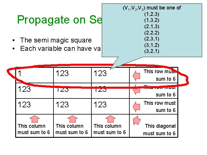
Propagate on Semi-magic Square • The semi magic square • Each variable can have value 1, 2 or 3 1 123 123 This row must sum to 6 This column must sum to 6 This diagonal must sum to 6

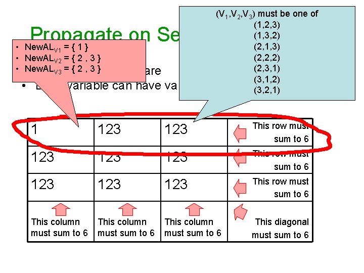
(V 1, V 2, V 3) must be one of (1, 2, 3) (1, 3, 2) (2, 1, 3) (2, 2, 2) (2, 3, 1) (3, 1, 2) 2 or 3 (3, 2, 1) Propagate on Semi-magic Square • The semi magic square • Each variable can have value 1, 1 123 123 This row must sum to 6 This column must sum to 6 This diagonal must sum to 6

(V 1, V 2, V 3) must be one of (1, 2, 3) (1, 3, 2) (2, 1, 3) (2, 2, 2) (2, 3, 1) (3, 1, 2) 2 or 3 (3, 2, 1) Propagate on Semi-magic Square • New. AL = { 1 } V 1 • New. ALV 2 = { 2 , 3 } • • New. AL = { 2 , magic 3} The. V 3 semi square • Each variable can have value 1, 1 123 123 This row must sum to 6 This column must sum to 6 This diagonal must sum to 6

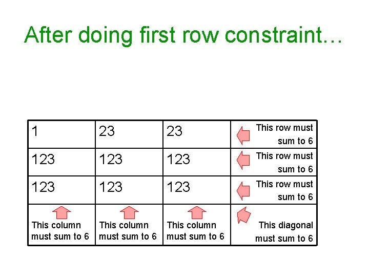
After doing first row constraint… 1 23 23 This row must sum to 6 123 123 123 This row must sum to 6 This column must sum to 6 This diagonal must sum to 6

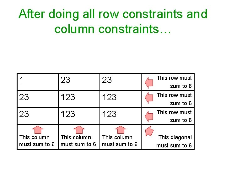
After doing all row constraints and column constraints… 1 23 23 This row must sum to 6 23 123 123 This row must sum to 6 This column must sum to 6 This diagonal must sum to 6

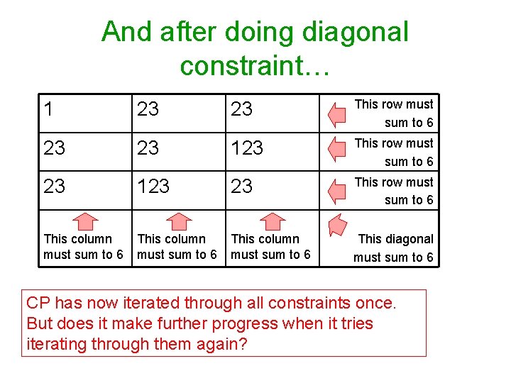
And after doing diagonal constraint… 1 23 23 This row must sum to 6 23 23 123 This row must sum to 6 23 123 23 This row must sum to 6 This column must sum to 6 This diagonal must sum to 6 CP has now iterated through all constraints once. But does it make further progress when it tries iterating through them again?

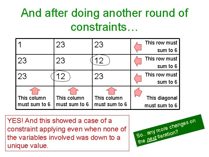
And after doing another round of constraints… 1 23 23 This row must sum to 6 23 23 12 This row must sum to 6 23 12 23 This row must sum to 6 This column must sum to 6 This diagonal must sum to 6 YES! And this showed a case of a constraint applying even when none of the variables involved was down to a unique value. n es o g n a re ch o m any ration? . . o S xt ite e n the

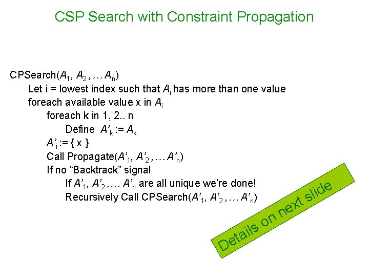
CSP Search with Constraint Propagation CPSearch(A 1, A 2 , … An) Let i = lowest index such that Ai has more than one value foreach available value x in Ai foreach k in 1, 2. . n Define A’k : = Ak A’i : = { x } Call Propagate(A’ 1, A’ 2 , … A’n) If no “Backtrack” signal If A’ 1, A’ 2 , … A’n are all unique we’re done! Recursively Call CPSearch(A’ 1, A’ 2 , … A’n) De s l i ta n n o t x e e d i l s

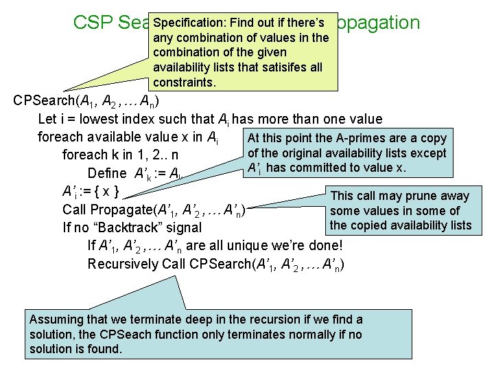
Specification: Find out if there’s CSP Search with Constraint Propagation any combination of values in the combination of the given availability lists that satisifes all constraints. CPSearch(A 1, A 2 , … An) Let i = lowest index such that Ai has more than one value foreach available value x in Ai At this point the A-primes are a copy of the original availability lists except foreach k in 1, 2. . n A’i has committed to value x. Define A’k : = Ak A’i : = { x } This call may prune away Call Propagate(A’ 1, A’ 2 , … A’n) some values in some of the copied availability lists If no “Backtrack” signal If A’ 1, A’ 2 , … A’n are all unique we’re done! Recursively Call CPSearch(A’ 1, A’ 2 , … A’n) Assuming that we terminate deep in the recursion if we find a solution, the CPSeach function only terminates normally if no solution is found.

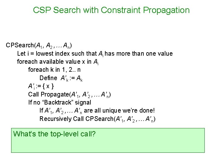
CSP Search with Constraint Propagation CPSearch(A 1, A 2 , … An) Let i = lowest index such that Ai has more than one value foreach available value x in Ai foreach k in 1, 2. . n Define A’k : = Ak A’i : = { x } Call Propagate(A’ 1, A’ 2 , … A’n) If no “Backtrack” signal If A’ 1, A’ 2 , … A’n are all unique we’re done! Recursively Call CPSearch(A’ 1, A’ 2 , … A’n) What’s the top-level call? Call with that Ai = complete set of possible values for Vi.

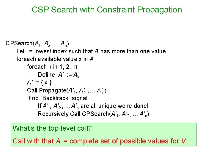
CSP Search with Constraint Propagation CPSearch(A 1, A 2 , … An) Let i = lowest index such that Ai has more than one value foreach available value x in Ai foreach k in 1, 2. . n Define A’k : = Ak A’i : = { x } Call Propagate(A’ 1, A’ 2 , … A’n) If no “Backtrack” signal If A’ 1, A’ 2 , … A’n are all unique we’re done! Recursively Call CPSearch(A’ 1, A’ 2 , … A’n) What’s the top-level call? Call with that Ai = complete set of possible values for Vi.

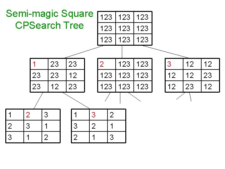
Semi-magic Square CPSearch Tree 1 23 23 1 23 23 12 3 1 2 23 1 3 2 123 123 123 2 123 123 3 2 1 3 3 12 12 23 12

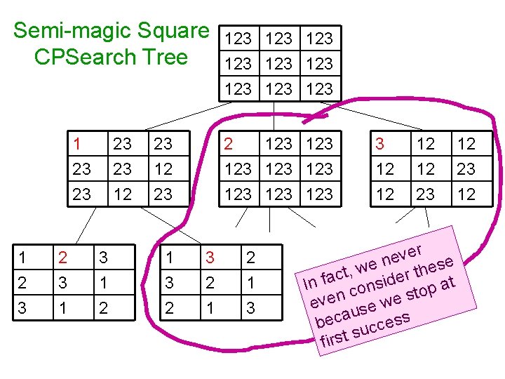
Semi-magic Square CPSearch Tree 1 23 23 1 23 23 12 3 1 2 23 1 3 2 123 123 123 2 123 123 3 2 1 3 3 12 12 23 ver e e n es we h , t t r c In fa conside op at t s n e e v w e e s u beca uccess if rst s 12 23 12

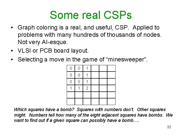
Some real CSPs • Graph coloring is a real, and useful, CSP. Applied to problems with many hundreds of thousands of nodes. Not very AI-esque. • VLSI or PCB board layout. • Selecting a move in the game of “minesweeper”. 0 0 1 1 1 2 Which squares have a bomb? Squares with numbers don’t. Other squares might. Numbers tell how many of the eight adjacent squares have bombs. We want to find out if a given square can possibly have a bomb…. 32

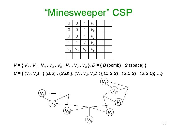
“Minesweeper” CSP 0 0 1 V 1 0 0 1 V 2 0 0 1 V 3 1 1 2 V 4 V 8 V 7 V 6 V 5 V = { V 1 , V 2 , V 3 , V 4 , V 5 , V 6 , V 7 , V 8 }, D = { B (bomb) , S (space) } C = { (V 1, V 2) : { (B, S) , (S, B) }, (V 1, V 2, V 3, ) : { (B, S, S) , (S, B, S) , (S, S, B)}, …} V 1 V 2 V 8 V 3 V 7 V 6 V 4 V 5 33

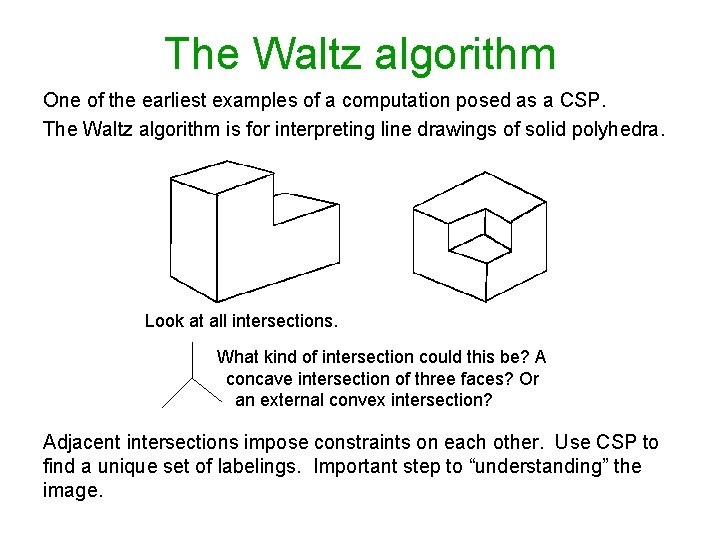
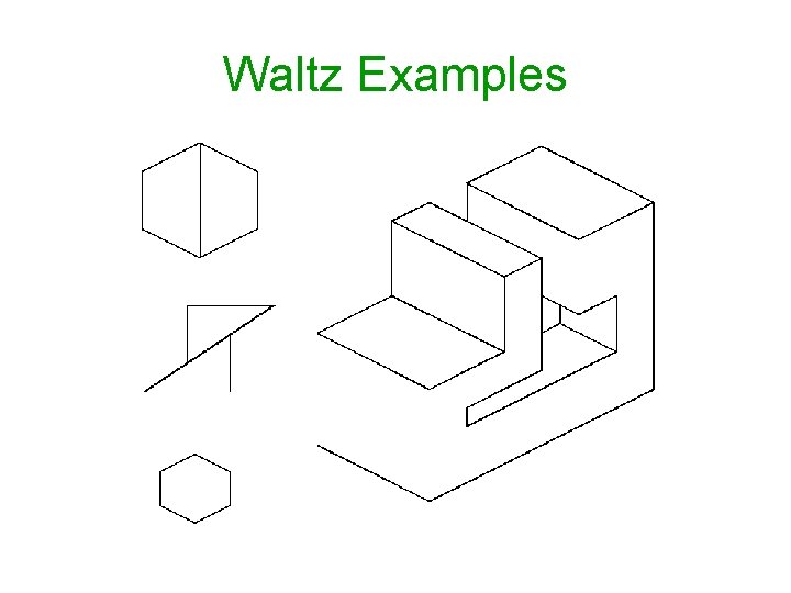
The Waltz algorithm One of the earliest examples of a computation posed as a CSP. The Waltz algorithm is for interpreting line drawings of solid polyhedra. Look at all intersections. What kind of intersection could this be? A concave intersection of three faces? Or an external convex intersection? Adjacent intersections impose constraints on each other. Use CSP to find a unique set of labelings. Important step to “understanding” the image.

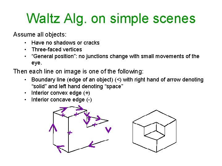
Waltz Alg. on simple scenes Assume all objects: • Have no shadows or cracks • Three-faced vertices • “General position”: no junctions change with small movements of the eye. Then each line on image is one of the following: • Boundary line (edge of an object) (<) with right hand of arrow denoting “solid” and left hand denoting “space” • Interior convex edge (+) • Interior concave edge (-)

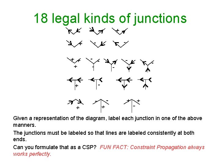
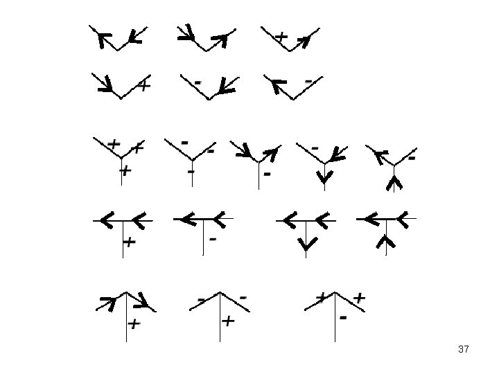
18 legal kinds of junctions Given a representation of the diagram, label each junction in one of the above manners. The junctions must be labeled so that lines are labeled consistently at both ends. Can you formulate that as a CSP? FUN FACT: Constraint Propagation always works perfectly.

37

Waltz Examples

Scheduling A very big, important use of CSP methods. • Used in many industries. Makes many multi-million dollar decisions. • Used extensively for space mission planning. • Military uses. People really care about improving scheduling algorithms! Problems with phenomenally huge state spaces. But for which solutions are needed very quickly. Many kinds of scheduling problems e. g. : v Job shop: Discrete time; weird ordering of operations possible; set of separate jobs. v Batch shop: Discrete or continuous time; restricted operation of ordering; grouping is important. v Manufacturing cell: Discrete, automated version of open job shop.

Job Shop scheduling At a job-shop you make various products. Each product is a “job” to be done. E. G. Job 1 = Make a polished-thing-with-a-hole Job 2 = Paint and drill a hole in a widget Each job requires several operations. E. G. Operations for Job 1: Polish, Drill Operations for Job 2: Paint, Drill Each operation needs several resources. E. G. Polishing needs the Polishing machine Polishing needs Pat (a Polishing expert) Drilling needs the Drilling needs Pat (also a Drilling expert) Or Drilling can be done by Chris Some operations need to be done in a particular order (e. g. Paint after you’ve Drilled)

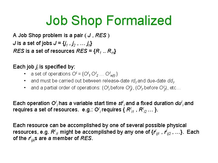
Job Shop Formalized A Job Shop problem is a pair ( J , RES ) J is a set of jobs J = {j 1 , j 2 , … jn} RES is a set of resources RES = {R 1. . Rm} Each job j. I is specified by: • • • a set of operations OI = {OI 1 OI 2 … OIn(I) } and must be carried out between release-date rd. I and due-date dd. I. and a partial order of operations: (OIi before OIj), (OIi’ before OIj’), etc… Each operation OIi has a variable start time st. Ii and a fixed duration du. Ii and requires a set of resources. e. g. : OIi requires { RIi 1 , RIi 2 … }. Each resource can be accomplished by one of several possible physical resources, e. g. RIi 1 might be accomplished by any one of {r. Iij 1 , r. Iij 2 , …}. Each of the r. Iijks are a member of RES.

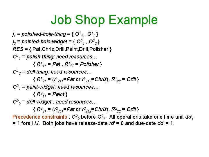
Job Shop Example j 1 = polished-hole-thing = { O 11 , O 12 } j 2 = painted-hole-widget = { O 21 , O 22 } RES = { Pat, Chris, Drill, Paint, Drill, Polisher } O 11 = polish-thing: need resources… { R 111 = Pat , R 112 = Polisher } O 12 = drill-thing: need resources… { R 121 = (r 1211=Pat or r 1212=Chris), R 122 = Drill } O 21 = paint-widget: need resources… { R 211 = Paint } O 22 = drill-widget : need resources… { R 221 = (r 2211=Pat or r 2212=Chris), R 222 = Drill } Precedence constraints : O 22 before O 21. All operations take one time unit du. Ii = 1 forall i, I. Both jobs have release-date rd. I = 0 and due-date dd. I = 1.

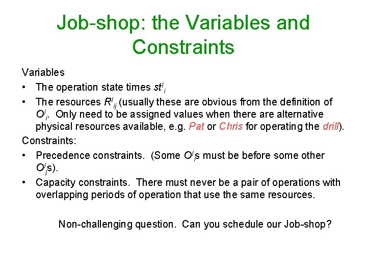
Job-shop: the Variables and Constraints Variables • The operation state times st. Ii • The resources RIij (usually these are obvious from the definition of OIi. Only need to be assigned values when there alternative physical resources available, e. g. Pat or Chris for operating the drill). Constraints: • Precedence constraints. (Some OIis must be before some other OIjs). • Capacity constraints. There must never be a pair of operations with overlapping periods of operation that use the same resources. Non-challenging question. Can you schedule our Job-shop?

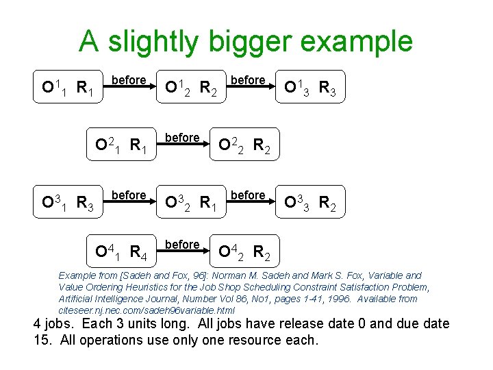
A slightly bigger example O 11 R 1 before O 21 R 1 O 31 R 3 before O 41 R 4 O 12 R 2 before O 32 R 1 before O 13 R 3 O 22 R 2 before O 33 R 2 O 42 R 2 Example from [Sadeh and Fox, 96]: Norman M. Sadeh and Mark S. Fox, Variable and Value Ordering Heuristics for the Job Shop Scheduling Constraint Satisfaction Problem, Artificial Intelligence Journal, Number Vol 86, No 1, pages 1 -41, 1996. Available from citeseer. nj. nec. com/sadeh 96 variable. html 4 jobs. Each 3 units long. All jobs have release date 0 and due date 15. All operations use only one resource each.

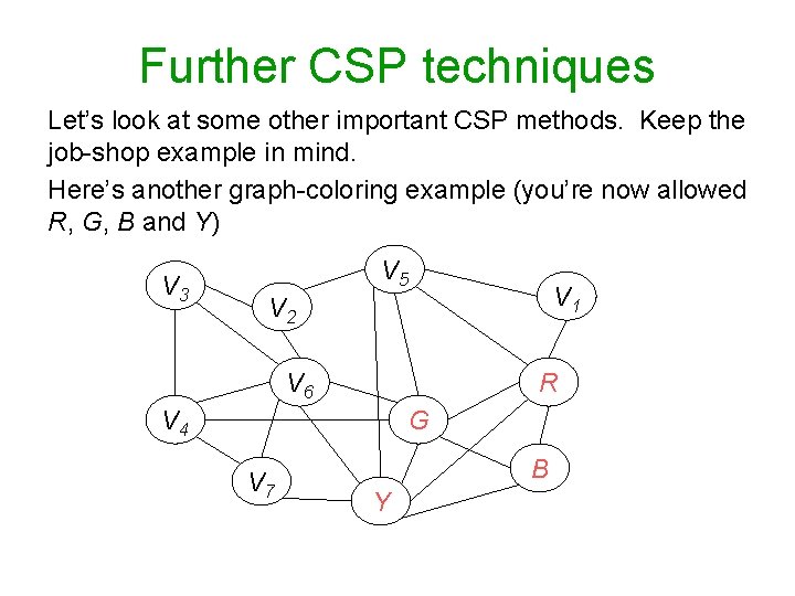
Further CSP techniques Let’s look at some other important CSP methods. Keep the job-shop example in mind. Here’s another graph-coloring example (you’re now allowed R, G, B and Y) V 3 V 5 V 1 V 2 V 6 R V 4 G V 7 B Y

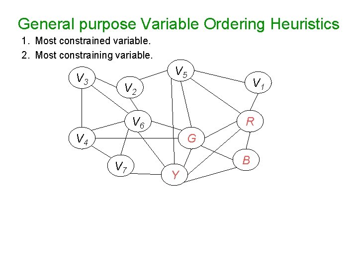
General purpose Variable Ordering Heuristics 1. Most constrained variable. 2. Most constraining variable. V 3 V 5 V 1 V 2 V 6 R V 4 G V 7 B Y

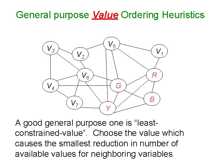
General purpose Value Ordering Heuristics V 3 V 5 V 1 V 2 V 6 R V 4 G V 7 B Y A good general purpose one is “leastconstrained-value”. Choose the value which causes the smallest reduction in number of available values for neighboring variables

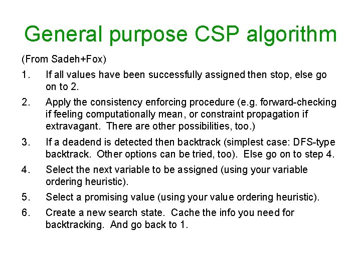
General purpose CSP algorithm (From Sadeh+Fox) 1. If all values have been successfully assigned then stop, else go on to 2. Apply the consistency enforcing procedure (e. g. forward-checking if feeling computationally mean, or constraint propagation if extravagant. There are other possibilities, too. ) 3. If a deadend is detected then backtrack (simplest case: DFS-type backtrack. Other options can be tried, too). Else go on to step 4. Select the next variable to be assigned (using your variable ordering heuristic). 5. Select a promising value (using your value ordering heuristic). 6. Create a new search state. Cache the info you need for backtracking. And go back to 1.

Job-shop example. Consistency enforcement Sadeh claims that generally forward-checking is better, computationally, than full constraint propagation. But it can be supplemented with a Job-shop specific TRICK. The precedence constraints (i. e. the available times for the operations to start due to the ordering of operations) can be computed exactly, given a partial schedule, very efficiently.

Reactive CSP solutions • Say you have built a large schedule. • Disaster! Halfway through execution, one of the resources breaks down. We have to reschedule! • Bad to have to wait 15 minutes for the scheduler to make a new suggestion. Important area of research: efficient schedule repair algorithms. • Question: If you expect that resources may sometimes break, what could a scheduling program do to take that into account? • Unrelated Question: Why has none of this lecture used A*?

Other approaches. And What You Should Know Other Approaches: Ø Hill-climbing, Tabu-search, Simulated annealing, Genetic Algorithms. (to be discussed later) What you should know: ü How to formalize problems as CSPs ü Backtracking Search, Forward Checking, Constraint Propagation ü The Waltz algorithm ü You should understand appreciate the way job-shop scheduling is formalized. It is an excellent representative example of how important well-studied constraint satisfaction problems are represented. ü Understand examples of Variable ordering and Value ordering heuristics In those cases where your lecturer or these handouts are too incomprehensible, consult Chap 5 of the Russell handout. Winston’s “Artificial Intelligence” book has good discussion of constraint satisfaction and Waltz algorithm.