Computational Intelligence Winter Term 201718 Prof Dr Gnter

Computational Intelligence Winter Term 2017/18 Prof. Dr. Günter Rudolph Lehrstuhl für Algorithm Engineering (LS 11) Fakultät für Informatik TU Dortmund

Plan for Today Lecture 06 ● Fuzzy sets § Axioms of fuzzy complement, t- and s-norms § Generators § Dual tripels G. Rudolph: Computational Intelligence ▪ Winter Term 2017/18 2

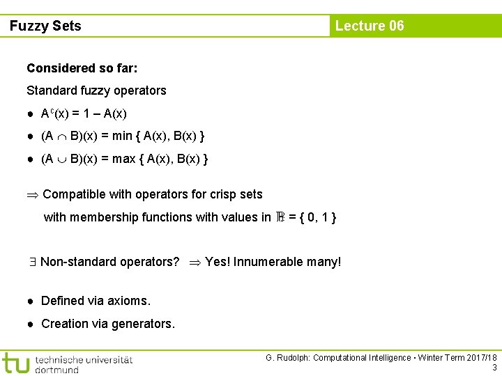
Fuzzy Sets Lecture 06 Considered so far: Standard fuzzy operators ● Ac(x) = 1 – A(x) ● (A B)(x) = min { A(x), B(x) } ● (A B)(x) = max { A(x), B(x) } Compatible with operators for crisp sets with membership functions with values in = { 0, 1 } Non-standard operators? Yes! Innumerable many! ● Defined via axioms. ● Creation via generators. G. Rudolph: Computational Intelligence ▪ Winter Term 2017/18 3

Fuzzy Complement: Axioms Lecture 06 Definition A function c: [0, 1] → [0, 1] is a fuzzy complement iff (A 1) c(0) = 1 and c(1) = 0. (A 2) a, b [0, 1]: a ≤ b c(a) ≥ c(b). monotone decreasing “nice to have”: (A 3) c(·) is continuous. (A 4) a [0, 1]: c(c(a)) = a involutive Examples: a) standard fuzzy complement c(a) = 1 – a ad (A 1): c(0) = 1 – 0 = 1 and c(1) = 1 – 1 = 0 ad (A 2): c‘(a) = – 1 < 0 (monotone decreasing) ad (A 3): ad (A 4): 1 – (1 – a) = a G. Rudolph: Computational Intelligence ▪ Winter Term 2017/18 4

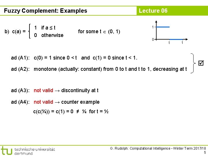
Fuzzy Complement: Examples b) c(a) = 1 if a ≤ t 0 otherwise Lecture 06 for some t (0, 1) 1 0 t 1 ad (A 1): c(0) = 1 since 0 < t and c(1) = 0 since t < 1. ad (A 2): monotone (actually: constant) from 0 to t and t to 1, decreasing at t ad (A 3): not valid → discontinuity at t ad (A 4): not valid → counter example c(c(¼)) = c(1) = 0 ≠ ¼ for t = ½ G. Rudolph: Computational Intelligence ▪ Winter Term 2017/18 5

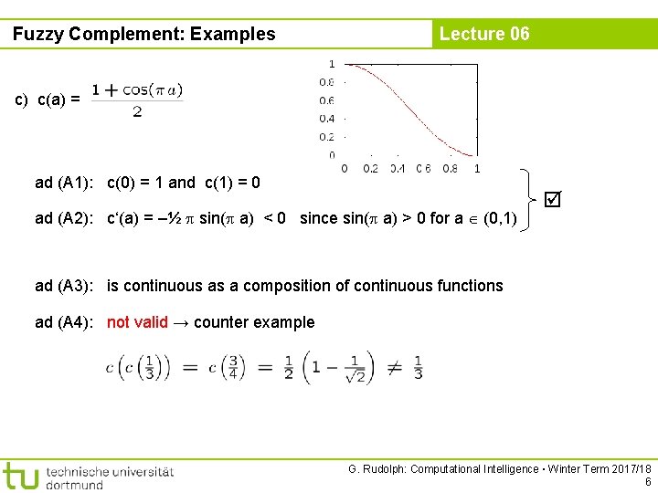
Fuzzy Complement: Examples Lecture 06 c) c(a) = ad (A 1): c(0) = 1 and c(1) = 0 ad (A 2): c‘(a) = –½ sin( a) < 0 since sin( a) > 0 for a (0, 1) ad (A 3): is continuous as a composition of continuous functions ad (A 4): not valid → counter example G. Rudolph: Computational Intelligence ▪ Winter Term 2017/18 6

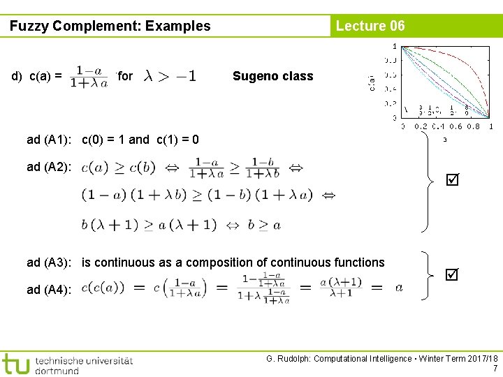
Fuzzy Complement: Examples d) c(a) = for Lecture 06 Sugeno class ad (A 1): c(0) = 1 and c(1) = 0 ad (A 2): ad (A 3): is continuous as a composition of continuous functions ad (A 4): G. Rudolph: Computational Intelligence ▪ Winter Term 2017/18 7

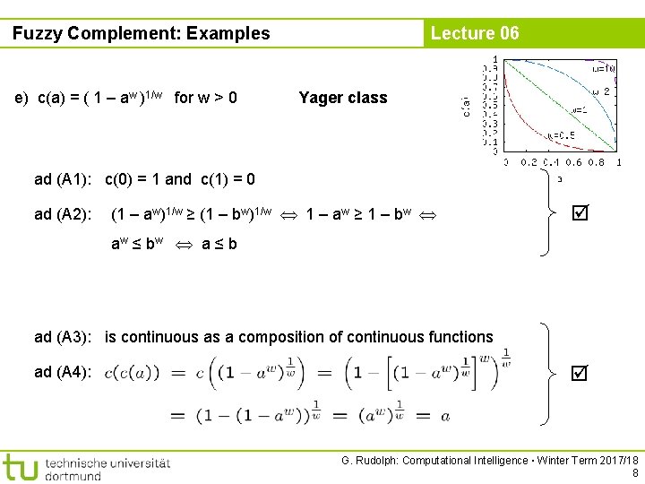
Fuzzy Complement: Examples e) c(a) = ( 1 – aw )1/w for w > 0 Lecture 06 Yager class ad (A 1): c(0) = 1 and c(1) = 0 ad (A 2): (1 – aw)1/w ≥ (1 – bw)1/w 1 – aw ≥ 1 – bw aw ≤ b w a ≤ b ad (A 3): is continuous as a composition of continuous functions ad (A 4): G. Rudolph: Computational Intelligence ▪ Winter Term 2017/18 8

Fuzzy Complement: Fixed Points Lecture 06 Theorem If function c: [0, 1] → [0, 1] satisfies axioms (A 1) and (A 2) of fuzzy complement then it has at most one fixed point a* with c(a*) = a*. Proof: one fixed point → see example (a) → intersection with bisectrix 1 0 1/2 1 t 1 1 no fixed point → see example (b) → no intersection with bisectrix 0 assume n > 1 fixed points, for example a* and b* with a* < b* c(a*) = a* and c(b*) = b* (fixed points) c(a*) < c(b*) with a* < b* impossible if c(·) is monotone decreasing contradiction to axiom (A 2) ■ G. Rudolph: Computational Intelligence ▪ Winter Term 2017/18 9

Fuzzy Complement: Fixed Points Lecture 06 Theorem If function c: [0, 1] → [0, 1] satisfies axioms (A 1) – (A 3) of fuzzy complement then it has exactly one fixed point a* with c(a*) = a*. Proof: Intermediate value theorem → If c(·) continuous (A 3) and c(0) ≥ c(1) (A 1/A 2) then v [c(1), c(0)] = [0, 1]: a [0, 1]: c(a) = v. there must be an intersection with bisectrix a fixed point exists and by previous theorem there are no other fixed points! ■ Examples: (a) c(a) = 1 – a a=1–a a* = ½ (b) c(a) = (1 – aw)1/w a* = (½)1/w G. Rudolph: Computational Intelligence ▪ Winter Term 2017/18 10

Fuzzy Complement: 1 st Characterization Lecture 06 Theorem c: [0, 1] → [0, 1] is involutive fuzzy complement iff continuous function g: [0, 1] → with defines an increasing generator • g(0) = 0 • strictly monotone increasing • a [0, 1]: c(a) = g(-1)( g(1) – g(a) ). ■ g(-1)(x) pseudo-inverse Examples a) g(x) = x g-1(x) = x c(a) = 1 – a (Standard) b) g(x) = xw g-1(x) = x 1/w c(a) = (1 – aw)1/w (Yager class, w > 0) c) g(x) = log(x+1) g-1(x) = ex – 1 c(a) = exp( log(2) – log(a+1) ) – 1 = 1–a 1+a (Sugeno class. = 1) G. Rudolph: Computational Intelligence ▪ Winter Term 2017/18 11

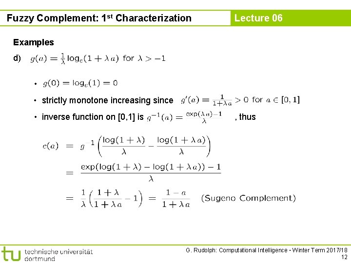
Fuzzy Complement: 1 st Characterization Lecture 06 Examples d) • • strictly monotone increasing since • inverse function on [0, 1] is , thus G. Rudolph: Computational Intelligence ▪ Winter Term 2017/18 12

Fuzzy Complement: 2 nd Characterization Lecture 06 Theorem c: [0, 1] → [0, 1] is involutive fuzzy complement iff continuous function f: [0, 1] → with defines a decreasing generator • f(1) = 0 • strictly monotone decreasing • a [0, 1]: c(a) = f(-1)( f(0) – f(a) ). ■ f(-1)(x) pseudo-inverse Examples a) f(x) = k – k · x (k > 0) f(-1)(x) = 1 – x/k c(a) = b) f(x) = 1 – xw f(-1)(x) = (1 – x)1/w c(a) = f-1(aw) = (1 – aw)1/w (Yager) G. Rudolph: Computational Intelligence ▪ Winter Term 2017/18 13

Fuzzy Intersection: t-norm Lecture 06 Definition A function t: [0, 1] x [0, 1] → [0, 1] is a fuzzy intersection or t-norm iff a, b, d [0, 1] (A 1) t(a, 1) = a (boundary condition) (A 2) b ≤ d t(a, b) ≤ t(a, d) (monotonicity) (A 3) t(a, b) = t(b, a) (commutative) (A 4) t(a, t(b, d)) = t(t(a, b), d) (associative) ■ “nice to have” (A 5) t(a, b) is continuous (A 6) t(a, a) < a (continuity) for 0 < a < 1 (subidempotent) (A 7) a 1 < a 2 and b 1 ≤ b 2 t(a 1, b 1) < t(a 2, b 2) (strict monotonicity) Note: the only idempotent t-norm is the standard fuzzy intersection G. Rudolph: Computational Intelligence ▪ Winter Term 2017/18 14

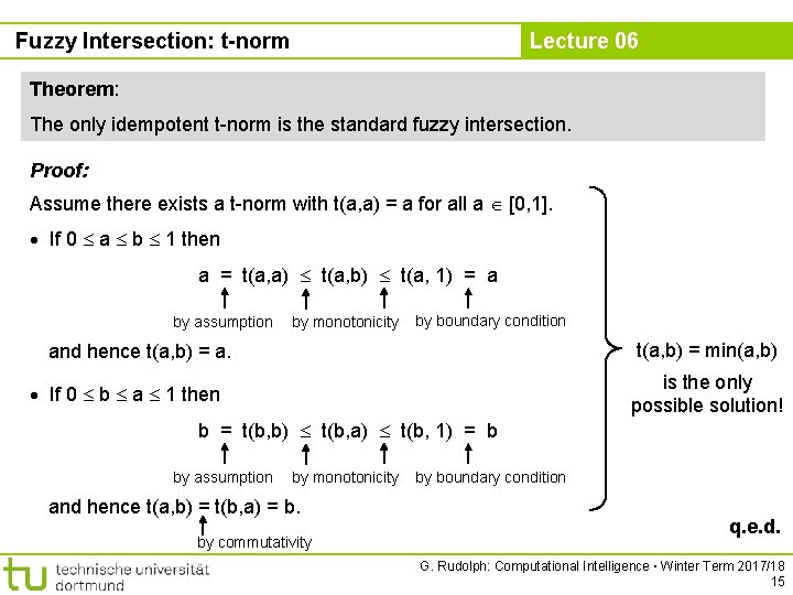
Fuzzy Intersection: t-norm Lecture 06 Theorem: The only idempotent t-norm is the standard fuzzy intersection. Proof: Assume there exists a t-norm with t(a, a) = a for all a [0, 1]. If 0 a b 1 then a = t(a, a) t(a, b) t(a, 1) = a by assumption by monotonicity by boundary condition t(a, b) = min(a, b) and hence t(a, b) = a. is the only possible solution! If 0 b a 1 then b = t(b, b) t(b, a) t(b, 1) = b by assumption by monotonicity and hence t(a, b) = t(b, a) = b. by commutativity by boundary condition q. e. d. G. Rudolph: Computational Intelligence ▪ Winter Term 2017/18 15

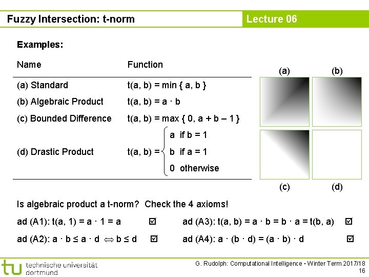
Fuzzy Intersection: t-norm Lecture 06 Examples: Name Function (a) Standard t(a, b) = min { a, b } (b) Algebraic Product t(a, b) = a · b (c) Bounded Difference t(a, b) = max { 0, a + b – 1 } (a) (b) (c) (d) a if b = 1 (d) Drastic Product t(a, b) = b if a = 1 0 otherwise Is algebraic product a t-norm? Check the 4 axioms! ad (A 1): t(a, 1) = a · 1 = a ad (A 3): t(a, b) = a · b = b · a = t(b, a) ad (A 2): a · b ≤ a · d b ≤ d ad (A 4): a · (b · d) = (a · b) · d G. Rudolph: Computational Intelligence ▪ Winter Term 2017/18 16

Fuzzy Intersection: Characterization Lecture 06 Theorem Function t: [0, 1] x [0, 1] → [0, 1] is a t-norm , decreasing generator f: [0, 1] → with t(a, b) = f-1( min{ f(0), f(a) + f(b) } ). ■ Example: f(x) = 1/x – 1 is decreasing generator since • f(x) is continuous • f(1) = 1/1 – 1 = 0 • f‘(x) = – 1/x 2 < 0 (monotone decreasing) inverse function is f-1(x) = ; f(0) = min{ f(0), f(a) + f(b) } = f(a) + f(b) t(a, b) = G. Rudolph: Computational Intelligence ▪ Winter Term 2017/18 17

Fuzzy Union: s-norm Lecture 06 Definition A function s: [0, 1] x [0, 1] → [0, 1] is a fuzzy union or s-norm iff a, b, d [0, 1] (A 1) s(a, 0) = a (boundary condition) (A 2) b ≤ d s(a, b) ≤ s(a, d) (monotonicity) (A 3) s(a, b) = s(b, a) (commutative) (A 4) s(a, s(b, d)) = s(s(a, b), d) (associative) ■ “nice to have” (A 5) s(a, b) is continuous (A 6) s(a, a) > a (continuity) for 0 < a < 1 (superidempotent) (A 7) a 1 < a 2 and b 1 ≤ b 2 s(a 1, b 1) < s(a 2, b 2) (strict monotonicity) Note: the only idempotent s-norm is the standard fuzzy union G. Rudolph: Computational Intelligence ▪ Winter Term 2017/18 18

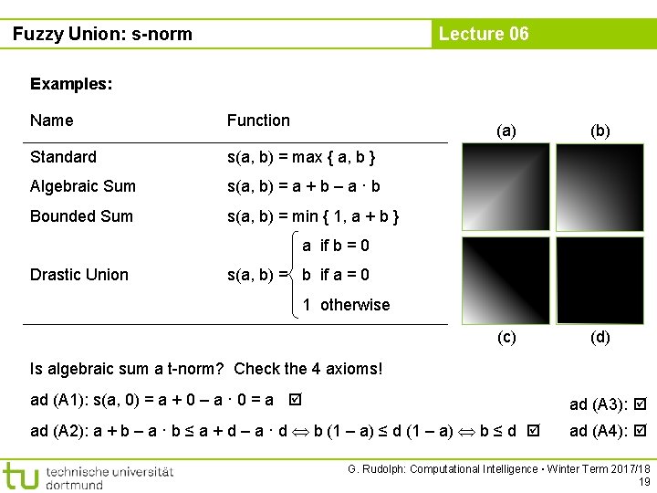
Fuzzy Union: s-norm Lecture 06 Examples: Name Function Standard s(a, b) = max { a, b } Algebraic Sum s(a, b) = a + b – a · b Bounded Sum s(a, b) = min { 1, a + b } (a) (b) (c) (d) a if b = 0 Drastic Union s(a, b) = b if a = 0 1 otherwise Is algebraic sum a t-norm? Check the 4 axioms! ad (A 1): s(a, 0) = a + 0 – a · 0 = a ad (A 3): ad (A 2): a + b – a · b ≤ a + d – a · d b (1 – a) ≤ d (1 – a) b ≤ d ad (A 4): G. Rudolph: Computational Intelligence ▪ Winter Term 2017/18 19

Fuzzy Union: Characterization Lecture 06 Theorem Function s: [0, 1] x [0, 1] → [0, 1] is a s-norm increasing generator g: [0, 1] → with s(a, b) = g-1( min{ g(1), g(a) + g(b) }). ■ Example: g(x) = –log(1 – x) is increasing generator since • g(x) is continuous • g(0) = –log(1 – 0) = 0 • g‘(x) = 1/(1 – x) > 0 (monotone increasing) inverse function is g-1(x) = 1 – exp(–x) ; g(1) = min{g(1), g(a) + g(b)} = g(a) + g(b) s(a, b) (algebraic sum) G. Rudolph: Computational Intelligence ▪ Winter Term 2017/18 20

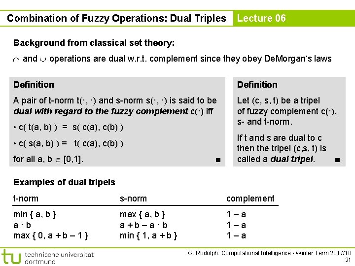
Combination of Fuzzy Operations: Dual Triples Lecture 06 Background from classical set theory: and operations are dual w. r. t. complement since they obey De. Morgan‘s laws Definition A pair of t-norm t(·, ·) and s-norm s(·, ·) is said to be dual with regard to the fuzzy complement c(·) iff Let (c, s, t) be a tripel of fuzzy complement c(·), s- and t-norm. • c( t(a, b) ) = s( c(a), c(b) ) • c( s(a, b) ) = t( c(a), c(b) ) for all a, b [0, 1]. ■ If t and s are dual to c then the tripel (c, s, t) is called a dual tripel. ■ Examples of dual tripels t-norm s-norm complement min { a, b } a·b max { 0, a + b – 1 } max { a, b } a+b–a·b min { 1, a + b } 1–a 1–a G. Rudolph: Computational Intelligence ▪ Winter Term 2017/18 21

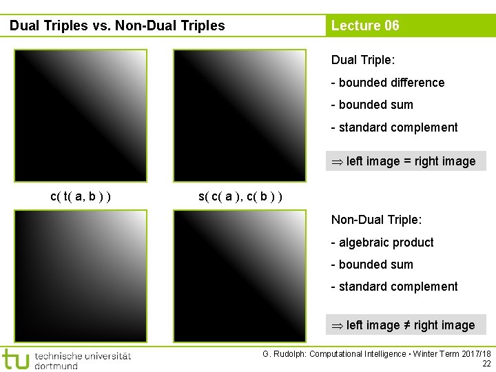
Dual Triples vs. Non-Dual Triples Lecture 06 Dual Triple: - bounded difference - bounded sum - standard complement left image = right image c( t( a, b ) ) s( c( a ), c( b ) ) Non-Dual Triple: - algebraic product - bounded sum - standard complement left image ≠ right image G. Rudolph: Computational Intelligence ▪ Winter Term 2017/18 22

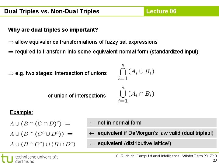
Dual Triples vs. Non-Dual Triples Lecture 06 Why are dual triples so important? allow equivalence transformations of fuzzy set expressions required to transform into some equivalent normal form (standardized input) e. g. two stages: intersection of unions or union of intersections Example: ← not in normal form ← equivalent if De. Morgan‘s law valid (dual triples!) ← equivalent (distributive lattice!) G. Rudolph: Computational Intelligence ▪ Winter Term 2017/18 23