Computational Intelligence Winter Term 201415 Prof Dr Gnter

Computational Intelligence Winter Term 2014/15 Prof. Dr. Günter Rudolph Lehrstuhl für Algorithm Engineering (LS 11) Fakultät für Informatik TU Dortmund

Plan for Today Lecture 06 ● Fuzzy sets § Axioms of fuzzy complement, t- and s-norms § Generators § Dual tripels G. Rudolph: Computational Intelligence ▪ Winter Term 2014/15 2

Fuzzy Sets Lecture 06 Considered so far: Standard fuzzy operators ● Ac(x) = 1 – A(x) ● (A Å B)(x) = min { A(x), B(x) } ● (A [ B)(x) = max { A(x), B(x) } ) Compatible with operators for crisp sets with membership functions with values in B = { 0, 1 } 9 Non-standard operators? ) Yes! Innumerable many! ● Defined via axioms. ● Creation via generators. G. Rudolph: Computational Intelligence ▪ Winter Term 2014/15 3

Fuzzy Complement: Axioms Lecture 06 Definition A function c: [0, 1] → [0, 1] is a fuzzy complement iff (A 1) c(0) = 1 and c(1) = 0. (A 2) 8 a, b 2 [0, 1]: a ≤ b ) c(a) ≥ c(b). monotone decreasing “nice to have”: (A 3) c(¢) is continuous. (A 4) 8 a 2 [0, 1]: c(c(a)) = a involutive Examples: a) standard fuzzy complement c(a) = 1 – a ad (A 1): c(0) = 1 – 0 = 1 and c(1) = 1 – 1 = 0 ad (A 2): c‘(a) = – 1 < 0 (monotone decreasing) ad (A 3): ad (A 4): 1 – (1 – a) = a G. Rudolph: Computational Intelligence ▪ Winter Term 2014/15 4

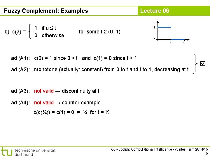
Fuzzy Complement: Examples b) c(a) = 1 if a ≤ t 0 otherwise Lecture 06 for some t 2 (0, 1) 1 0 t 1 ad (A 1): c(0) = 1 since 0 < t and c(1) = 0 since t < 1. ad (A 2): monotone (actually: constant) from 0 to t and t to 1, decreasing at t ad (A 3): not valid → discontinuity at t ad (A 4): not valid → counter example c(c(¼)) = c(1) = 0 ≠ ¼ for t = ½ G. Rudolph: Computational Intelligence ▪ Winter Term 2014/15 5

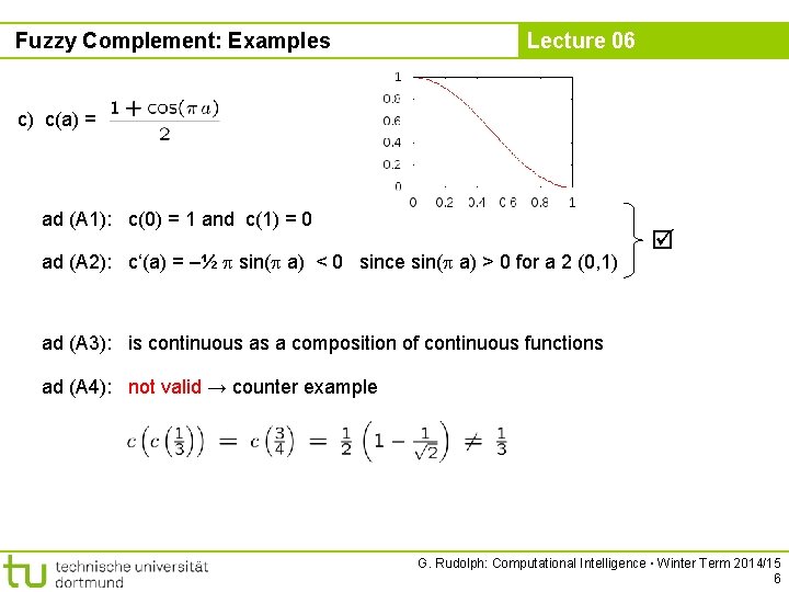
Fuzzy Complement: Examples Lecture 06 c) c(a) = ad (A 1): c(0) = 1 and c(1) = 0 ad (A 2): c‘(a) = –½ sin( a) < 0 since sin( a) > 0 for a 2 (0, 1) ad (A 3): is continuous as a composition of continuous functions ad (A 4): not valid → counter example G. Rudolph: Computational Intelligence ▪ Winter Term 2014/15 6

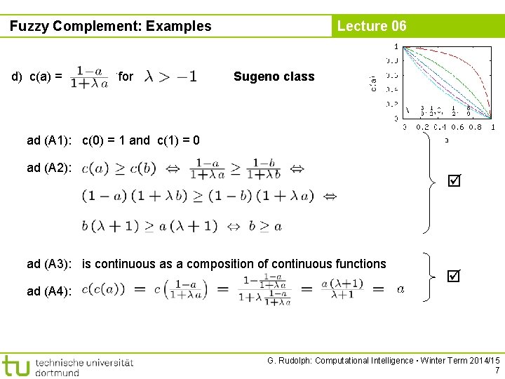
Fuzzy Complement: Examples d) c(a) = for Lecture 06 Sugeno class ad (A 1): c(0) = 1 and c(1) = 0 ad (A 2): ad (A 3): is continuous as a composition of continuous functions ad (A 4): G. Rudolph: Computational Intelligence ▪ Winter Term 2014/15 7

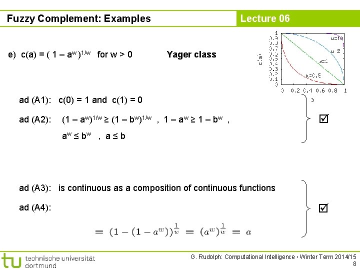
Fuzzy Complement: Examples e) c(a) = ( 1 – aw )1/w for w > 0 Lecture 06 Yager class ad (A 1): c(0) = 1 and c(1) = 0 ad (A 2): (1 – aw)1/w ≥ (1 – bw)1/w , 1 – aw ≥ 1 – bw , aw ≤ b w , a ≤ b ad (A 3): is continuous as a composition of continuous functions ad (A 4): G. Rudolph: Computational Intelligence ▪ Winter Term 2014/15 8

Fuzzy Complement: Fixed Points Lecture 06 Theorem If function c: [0, 1] → [0, 1] satisfies axioms (A 1) and (A 2) of fuzzy complement then it has at most one fixed point a* with c(a*) = a*. Proof: one fixed point → see example (a) → intersection with bisectrix 1 0 1/2 1 t 1 1 no fixed point → see example (b) → no intersection with bisectrix 0 assume 9 n > 1 fixed points, for example a* and b* with a* < b* ) c(a*) = a* and c(b*) = b* (fixed points) ) c(a*) < c(b*) with a* < b* impossible if c(¢) is monotone decreasing ) contradiction to axiom (A 2) ■ G. Rudolph: Computational Intelligence ▪ Winter Term 2014/15 9

Fuzzy Complement: Fixed Points Lecture 06 Theorem If function c: [0, 1] → [0, 1] satisfies axioms (A 1) – (A 3) of fuzzy complement then it has exactly one fixed point a* with c(a*) = a*. Proof: Intermediate value theorem → If c(¢) continuous (A 3) and c(0) ≥ c(1) (A 1/A 2) then 8 v 2 [c(1), c(0)] = [0, 1]: 9 a 2 [0, 1]: c(a) = v. ) there must be an intersection with bisectrix ) a fixed point exists and by previous theorem there are no other fixed points! ■ Examples: (a) c(a) = 1 – a )a=1–a ) a* = ½ (b) c(a) = (1 – aw)1/w ) a* = (½)1/w G. Rudolph: Computational Intelligence ▪ Winter Term 2014/15 10

Fuzzy Complement: 1 st Characterization Lecture 06 Theorem c: [0, 1] → [0, 1] is involutive fuzzy complement iff 9 continuous function g: [0, 1] → R with defines an increasing generator • g(0) = 0 • strictly monotone increasing • 8 a 2 [0, 1]: c(a) = g(-1)( g(1) – g(a) ). ■ g(-1)(x) pseudo-inverse Examples a) g(x) = x ) g-1(x) = x ) c(a) = 1 – a b) g(x) = xw ) g-1(x) = x 1/w ) c(a) = (1 – aw)1/w (Yager class, w > 0) c) g(x) = log(x+1) ) g-1(x) = ex – 1 (Standard) ) c(a) = exp( log(2) – log(a+1) ) – 1 = 1–a 1+a (Sugeno class. = 1) G. Rudolph: Computational Intelligence ▪ Winter Term 2014/15 11

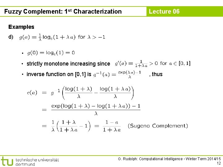
Fuzzy Complement: 1 st Characterization Lecture 06 Examples d) • • strictly monotone increasing since • inverse function on [0, 1] is , thus G. Rudolph: Computational Intelligence ▪ Winter Term 2014/15 12

Fuzzy Complement: 2 nd Characterization Lecture 06 Theorem c: [0, 1] → [0, 1] is involutive fuzzy complement iff 9 continuous function f: [0, 1] → R with defines a decreasing generator • f(1) = 0 • strictly monotone decreasing • 8 a 2 [0, 1]: c(a) = f(-1)( f(0) – f(a) ). ■ f(-1)(x) pseudo-inverse Examples a) f(x) = k – k ¢ x (k > 0) f(-1)(x) = 1 – x/k c(a) = b) f(x) = 1 – xw c(a) = f-1(aw) = (1 – aw)1/w f(-1)(x) = (1 – x)1/´w (Yager) G. Rudolph: Computational Intelligence ▪ Winter Term 2014/15 13

Fuzzy Intersection: t-norm Lecture 06 Definition A function t: [0, 1] £ [0, 1] → [0, 1] is a fuzzy intersection or t-norm iff (A 1) t(a, 1) = a (A 2) b ≤ d ) t(a, b) ≤ t(a, d) (monotonicity) (A 3) t(a, b) = t(b, a) (commutative) (A 4) t(a, t(b, d)) = t(t(a, b), d) (associative) ■ “nice to have” (A 5) t(a, b) is continuous (continuity) (A 6) t(a, a) < a (subidempotent) (A 7) a 1 < a 2 and b 1 ≤ b 2 ) t(a 1, b 1) < t(a 2, b 2) (strict monotonicity) Note: the only idempotent t-norm is the standard fuzzy intersection G. Rudolph: Computational Intelligence ▪ Winter Term 2014/15 14

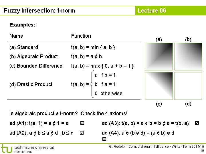
Fuzzy Intersection: t-norm Lecture 06 Examples: Name Function (a) Standard t(a, b) = min { a, b } (b) Algebraic Product t(a, b) = a ¢ b (c) Bounded Difference t(a, b) = max { 0, a + b – 1 } (a) (b) (c) (d) a if b = 1 (d) Drastic Product t(a, b) = b if a = 1 0 otherwise Is algebraic product a t-norm? Check the 4 axioms! ad (A 1): t(a, 1) = a ¢ 1 = a ad (A 3): t(a, b) = a ¢ b = b ¢ a = t(b, a) ad (A 2): a ¢ b ≤ a ¢ d , b ≤ d ad (A 4): a ¢ (b ¢ d) = (a ¢ b) ¢ d G. Rudolph: Computational Intelligence ▪ Winter Term 2014/15 15

Fuzzy Intersection: Characterization Lecture 06 Theorem Function t: [0, 1] £ [0, 1] → [0, 1] is a t-norm , 9 decreasing generator f: [0, 1] → R with t(a, b) = f(-1)( f(a) + f(b) ). ■ Example: f(x) = 1/x – 1 is decreasing generator since • f(x) is continuous • f(1) = 1/1 – 1 = 0 • f‘(x) = – 1/x 2 < 0 (monotone decreasing) inverse function is f-1(x) = ) t(a, b) = G. Rudolph: Computational Intelligence ▪ Winter Term 2014/15 16

Fuzzy Union: s-norm Lecture 06 Definition A function s: [0, 1] £ [0, 1] → [0, 1] is a fuzzy union or s-norm or t-conorm iff (A 1) s(a, 0) = a (A 2) b ≤ d ) s(a, b) ≤ s(a, d) (monotonicity) (A 3) s(a, b) = s(b, a) (commutative) (A 4) s(a, s(b, d)) = s(s(a, b), d) (associative) ■ “nice to have” (A 5) s(a, b) is continuous (continuity) (A 6) s(a, a) > a (superidempotent) (A 7) a 1 < a 2 and b 1 ≤ b 2 ) s(a 1, b 1) < s(a 2, b 2) (strict monotonicity) Note: the only idempotent s-norm is the standard fuzzy union G. Rudolph: Computational Intelligence ▪ Winter Term 2014/15 17

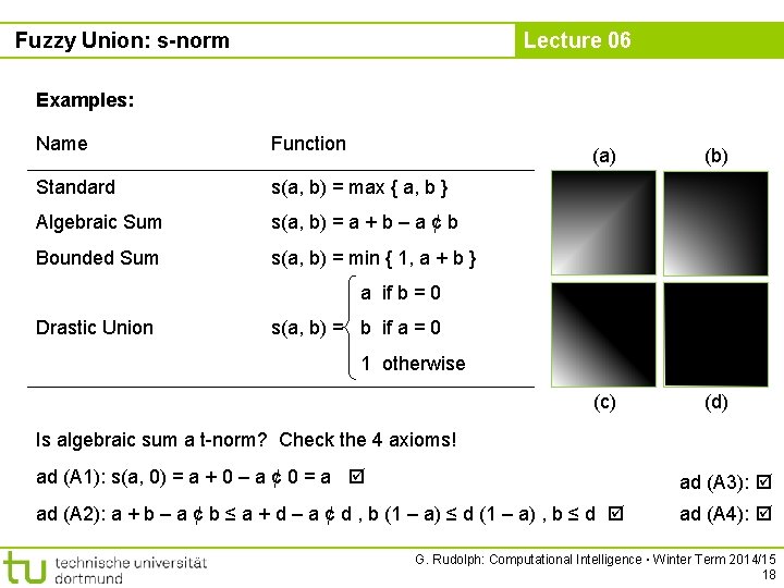
Fuzzy Union: s-norm Lecture 06 Examples: Name Function Standard s(a, b) = max { a, b } Algebraic Sum s(a, b) = a + b – a ¢ b Bounded Sum s(a, b) = min { 1, a + b } (a) (b) (c) (d) a if b = 0 Drastic Union s(a, b) = b if a = 0 1 otherwise Is algebraic sum a t-norm? Check the 4 axioms! ad (A 1): s(a, 0) = a + 0 – a ¢ 0 = a ad (A 3): ad (A 2): a + b – a ¢ b ≤ a + d – a ¢ d , b (1 – a) ≤ d (1 – a) , b ≤ d ad (A 4): G. Rudolph: Computational Intelligence ▪ Winter Term 2014/15 18

Fuzzy Union: Characterization Lecture 06 Theorem Function s: [0, 1] £ [0, 1] → [0, 1] is a s-norm , 9 increasing generator g: [0, 1] → R with s(a, b) = g(-1)( g(a) + g(b) ). ■ Example: g(x) = –log(1 – x) is increasing generator since • g(x) is continuous • g(0) = –log(1 – 0) = 0 • g‘(x) = 1/(1 – x) > 0 (monotone increasing) inverse function is g-1(x) = 1 – exp(–x) ) s(a, b) (algebraic sum) G. Rudolph: Computational Intelligence ▪ Winter Term 2014/15 19

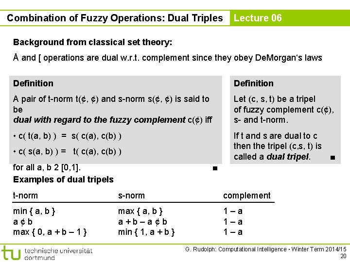
Combination of Fuzzy Operations: Dual Triples Lecture 06 Background from classical set theory: Å and [ operations are dual w. r. t. complement since they obey De. Morgan‘s laws Definition A pair of t-norm t(¢, ¢) and s-norm s(¢, ¢) is said to be dual with regard to the fuzzy complement c(¢) iff Let (c, s, t) be a tripel of fuzzy complement c(¢), s- and t-norm. • c( t(a, b) ) = s( c(a), c(b) ) If t and s are dual to c then the tripel (c, s, t) is called a dual tripel. ■ • c( s(a, b) ) = t( c(a), c(b) ) for all a, b 2 [0, 1]. Examples of dual tripels ■ t-norm s-norm complement min { a, b } a¢b max { 0, a + b – 1 } max { a, b } a+b–a¢b min { 1, a + b } 1–a 1–a G. Rudolph: Computational Intelligence ▪ Winter Term 2014/15 20

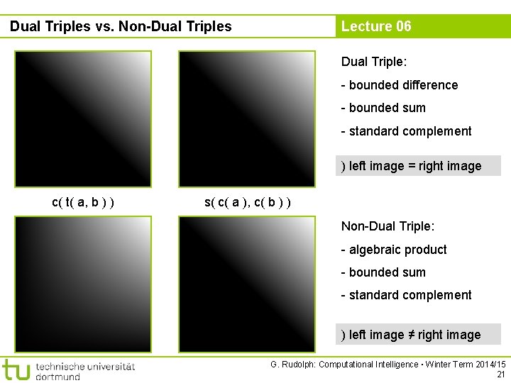
Dual Triples vs. Non-Dual Triples Lecture 06 Dual Triple: - bounded difference - bounded sum - standard complement ) left image = right image c( t( a, b ) ) s( c( a ), c( b ) ) Non-Dual Triple: - algebraic product - bounded sum - standard complement ) left image ≠ right image G. Rudolph: Computational Intelligence ▪ Winter Term 2014/15 21

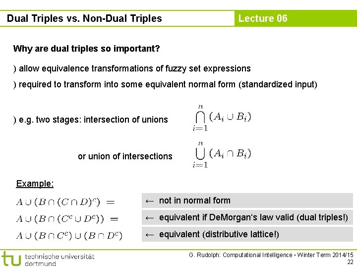
Dual Triples vs. Non-Dual Triples Lecture 06 Why are dual triples so important? ) allow equivalence transformations of fuzzy set expressions ) required to transform into some equivalent normal form (standardized input) ) e. g. two stages: intersection of unions or union of intersections Example: ← not in normal form ← equivalent if De. Morgan‘s law valid (dual triples!) ← equivalent (distributive lattice!) G. Rudolph: Computational Intelligence ▪ Winter Term 2014/15 22