Computational Intelligence Winter Term 201213 Prof Dr Gnter

Computational Intelligence Winter Term 2012/13 Prof. Dr. Günter Rudolph Lehrstuhl für Algorithm Engineering (LS 11) Fakultät für Informatik TU Dortmund

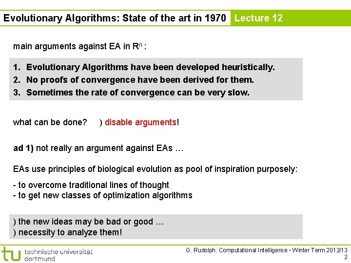
Evolutionary Algorithms: State of the art in 1970 Lecture 12 main arguments against EA in Rn : 1. Evolutionary Algorithms have been developed heuristically. 2. No proofs of convergence have been derived for them. 3. Sometimes the rate of convergence can be very slow. what can be done? ) disable arguments! ad 1) not really an argument against EAs … EAs use principles of biological evolution as pool of inspiration purposely: - to overcome traditional lines of thought - to get new classes of optimization algorithms ) the new ideas may be bad or good … ) necessity to analyze them! G. Rudolph: Computational Intelligence ▪ Winter Term 2012/13 2

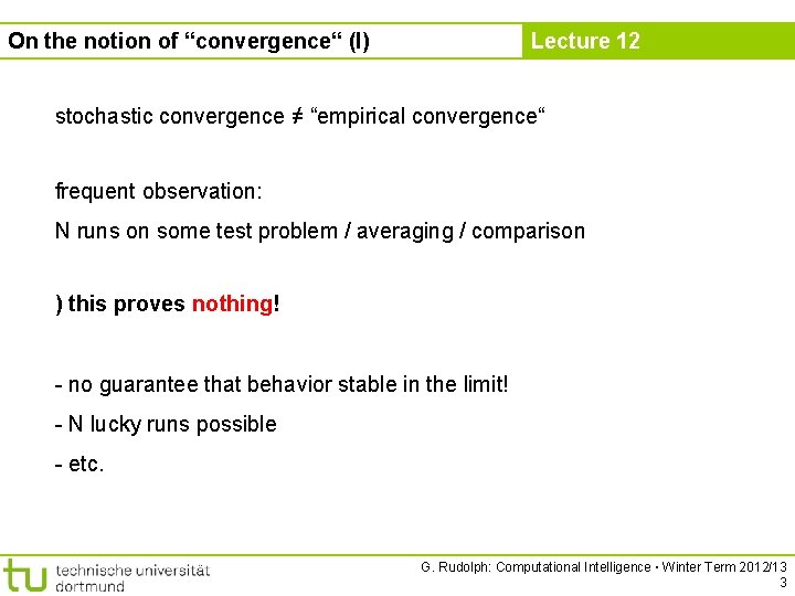
On the notion of “convergence“ (I) Lecture 12 stochastic convergence ≠ “empirical convergence“ frequent observation: N runs on some test problem / averaging / comparison ) this proves nothing! - no guarantee that behavior stable in the limit! - N lucky runs possible - etc. G. Rudolph: Computational Intelligence ▪ Winter Term 2012/13 3

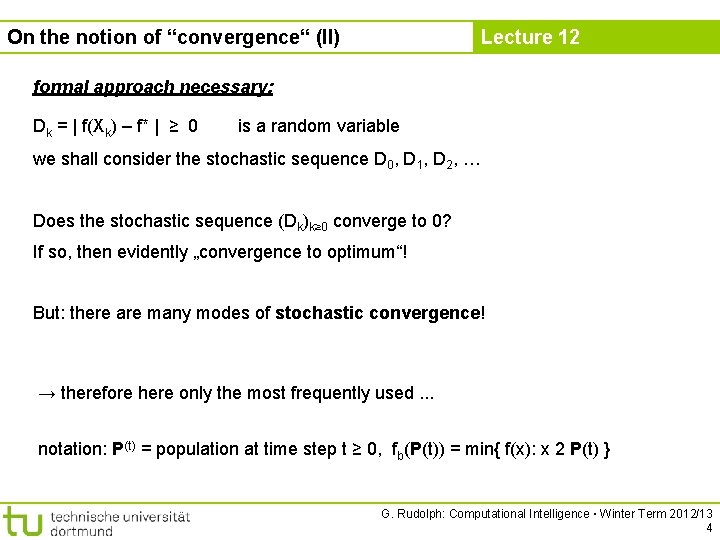
On the notion of “convergence“ (II) Lecture 12 formal approach necessary: Dk = | f(Xk) – f* | ≥ 0 is a random variable we shall consider the stochastic sequence D 0, D 1, D 2, … Does the stochastic sequence (Dk)k≥ 0 converge to 0? If so, then evidently „convergence to optimum“! But: there are many modes of stochastic convergence! → therefore here only the most frequently used. . . notation: P(t) = population at time step t ≥ 0, fb(P(t)) = min{ f(x): x 2 P(t) } G. Rudolph: Computational Intelligence ▪ Winter Term 2012/13 4

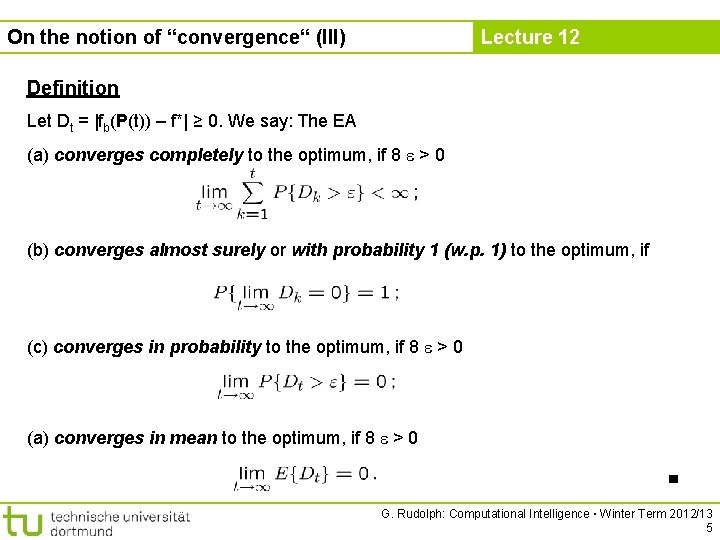
On the notion of “convergence“ (III) Lecture 12 Definition Let Dt = |fb(P(t)) – f*| ≥ 0. We say: The EA (a) converges completely to the optimum, if 8 > 0 (b) converges almost surely or with probability 1 (w. p. 1) to the optimum, if (c) converges in probability to the optimum, if 8 > 0 (a) converges in mean to the optimum, if 8 > 0 ■ G. Rudolph: Computational Intelligence ▪ Winter Term 2012/13 5

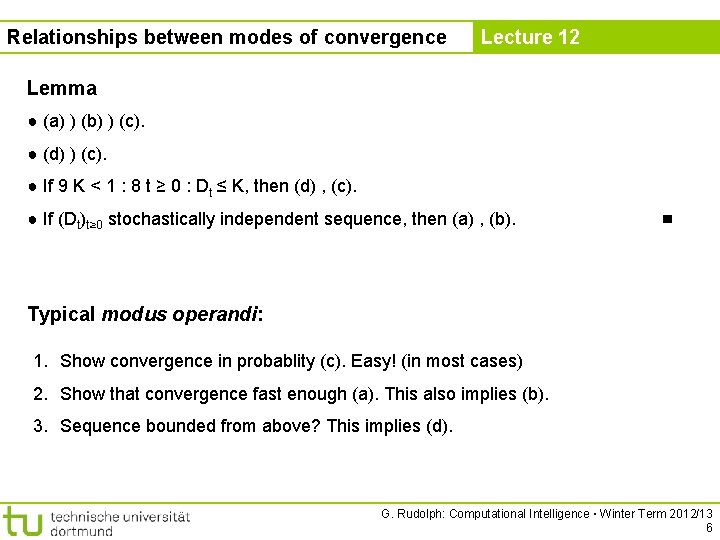
Relationships between modes of convergence Lecture 12 Lemma ● (a) ) (b) ) (c). ● (d) ) (c). ● If 9 K < 1 : 8 t ≥ 0 : Dt ≤ K, then (d) , (c). ● If (Dt)t≥ 0 stochastically independent sequence, then (a) , (b). ■ Typical modus operandi: 1. Show convergence in probablity (c). Easy! (in most cases) 2. Show that convergence fast enough (a). This also implies (b). 3. Sequence bounded from above? This implies (d). G. Rudolph: Computational Intelligence ▪ Winter Term 2012/13 6

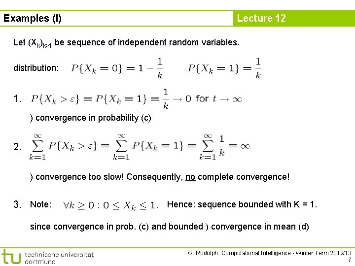
Examples (I) Lecture 12 Let (Xk)k≥ 1 be sequence of independent random variables. distribution: 1. ) convergence in probability (c) 2. ) convergence too slow! Consequently, no complete convergence! 3. Note: Hence: sequence bounded with K = 1. since convergence in prob. (c) and bounded ) convergence in mean (d) G. Rudolph: Computational Intelligence ▪ Winter Term 2012/13 7

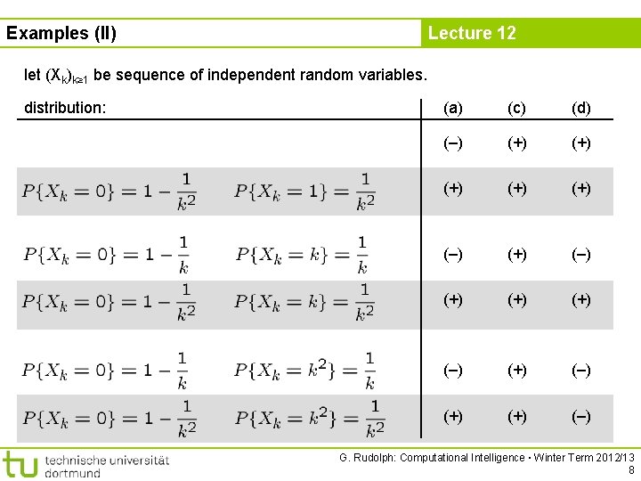
Examples (II) Lecture 12 let (Xk)k≥ 1 be sequence of independent random variables. distribution: (a) (c) (d) (–) (+) (+) (+) (–) (+) (+) (–) G. Rudolph: Computational Intelligence ▪ Winter Term 2012/13 8

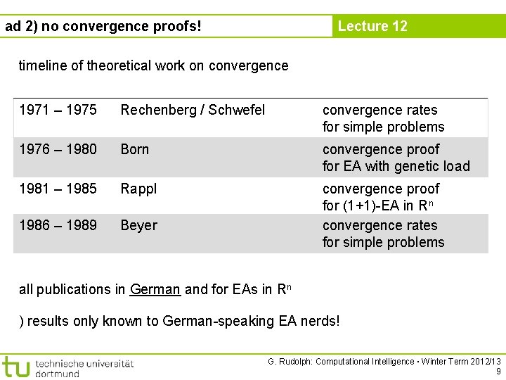
Lecture 12 ad 2) no convergence proofs! timeline of theoretical work on convergence 1971 – 1975 Rechenberg / Schwefel convergence rates for simple problems 1976 – 1980 Born convergence proof for EA with genetic load 1981 – 1985 Rappl 1986 – 1989 Beyer convergence proof for (1+1)-EA in Rn convergence rates for simple problems all publications in German and for EAs in Rn ) results only known to German-speaking EA nerds! G. Rudolph: Computational Intelligence ▪ Winter Term 2012/13 9

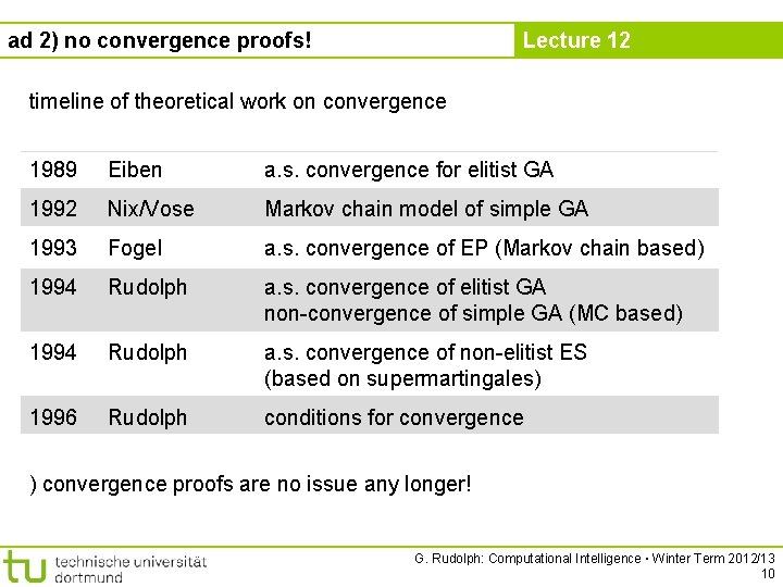
Lecture 12 ad 2) no convergence proofs! timeline of theoretical work on convergence 1989 Eiben a. s. convergence for elitist GA 1992 Nix/Vose Markov chain model of simple GA 1993 Fogel a. s. convergence of EP (Markov chain based) 1994 Rudolph a. s. convergence of elitist GA non-convergence of simple GA (MC based) 1994 Rudolph a. s. convergence of non-elitist ES (based on supermartingales) 1996 Rudolph conditions for convergence ) convergence proofs are no issue any longer! G. Rudolph: Computational Intelligence ▪ Winter Term 2012/13 10

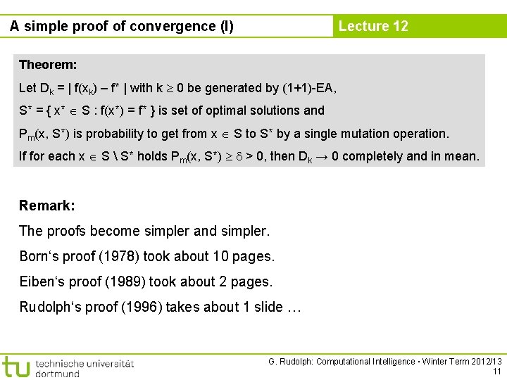
A simple proof of convergence (I) Lecture 12 Theorem: Let Dk = | f(xk) – f* | with k 0 be generated by (1+1)-EA, S* = { x* S : f(x*) = f* } is set of optimal solutions and Pm(x, S*) is probability to get from x S to S* by a single mutation operation. If for each x S S* holds Pm(x, S*) > 0, then Dk → 0 completely and in mean. Remark: The proofs become simpler and simpler. Born‘s proof (1978) took about 10 pages. Eiben‘s proof (1989) took about 2 pages. Rudolph‘s proof (1996) takes about 1 slide … G. Rudolph: Computational Intelligence ▪ Winter Term 2012/13 11

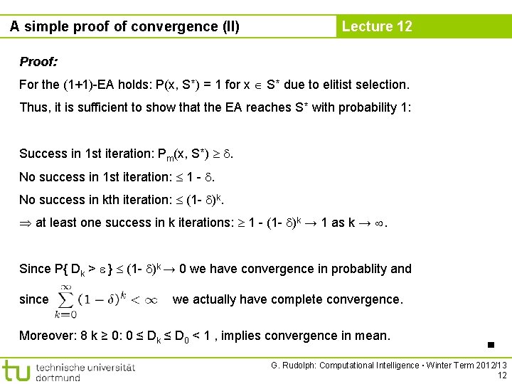
A simple proof of convergence (II) Lecture 12 Proof: For the (1+1)-EA holds: P(x, S*) = 1 for x S* due to elitist selection. Thus, it is sufficient to show that the EA reaches S* with probability 1: Success in 1 st iteration: Pm(x, S*) . No success in 1 st iteration: 1 - . No success in kth iteration: (1 - )k. at least one success in k iterations: 1 - (1 - )k → 1 as k → . Since P{ Dk > } (1 - )k → 0 we have convergence in probablity and since we actually have complete convergence. Moreover: 8 k ≥ 0: 0 ≤ Dk ≤ D 0 < 1 , implies convergence in mean. ■ G. Rudolph: Computational Intelligence ▪ Winter Term 2012/13 12

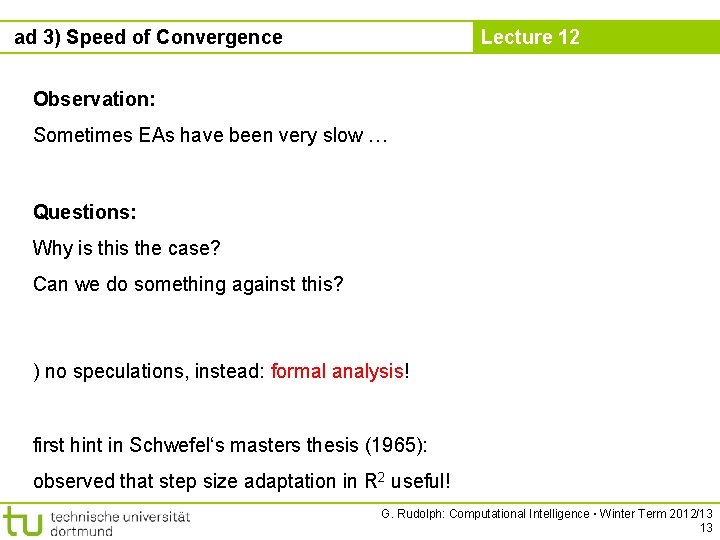
ad 3) Speed of Convergence Lecture 12 Observation: Sometimes EAs have been very slow … Questions: Why is the case? Can we do something against this? ) no speculations, instead: formal analysis! first hint in Schwefel‘s masters thesis (1965): observed that step size adaptation in R 2 useful! G. Rudolph: Computational Intelligence ▪ Winter Term 2012/13 13

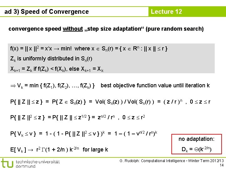
ad 3) Speed of Convergence Lecture 12 convergence speed without „step size adaptation“ (pure random search) f(x) = || x ||2 = x‘x → min! where x Sn(r) = { x Rn : || x || r } Zk is uniformly distributed in Sn(r) Xk+1 = Zk if f(Zk) < f(Xk), else Xk+1 = Xk Vk = min { f(Z 1), f(Z 2), …, f(Zk) } best objective function value until iteration k P{ || Z || z } = P{ Z Sn(z) } = Vol( Sn(z) ) / Vol( Sn(r) ) = ( z / r )n , 0 z r P{ || Z ||2 z } = P{ || Z || z 1/2 } = zn/2 / rn , 0 z r 2 P{ Vk v } = 1 - ( 1 - P{ || Z ||2 v } )k = 1 – ( 1 – vn/2 / rn)k E[ Vk ] → r 2 (1 + 2/n ) k-2/n for large k no adaptation: Dk = (k-2/n) G. Rudolph: Computational Intelligence ▪ Winter Term 2012/13 14

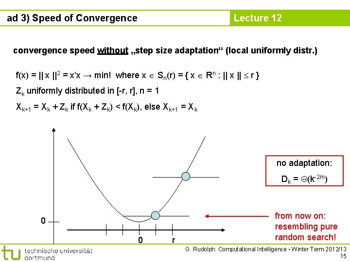
ad 3) Speed of Convergence Lecture 12 convergence speed without „step size adaptation“ (local uniformly distr. ) f(x) = || x ||2 = x‘x → min! where x Sn(r) = { x Rn : || x || r } Zk uniformly distributed in [-r, r], n = 1 Xk+1 = Xk + Zk if f(Xk + Zk) < f(Xk), else Xk+1 = Xk no adaptation: Dk = (k-2/n) 0 0 r from now on: resembling pure random search! G. Rudolph: Computational Intelligence ▪ Winter Term 2012/13 15

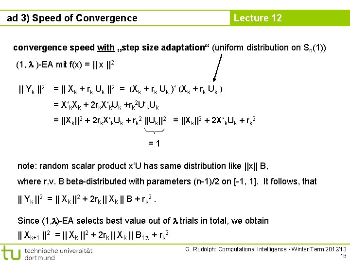
ad 3) Speed of Convergence Lecture 12 convergence speed with „step size adaptation“ (uniform distribution on Sn(1)) (1, )-EA mit f(x) = || x ||2 || Yk ||2 = || Xk + rk Uk ||2 = (Xk + rk Uk )‘ (Xk + rk Uk ) = X‘k. Xk + 2 rk. X‘k. Uk +rk 2 U‘k. Uk = ||Xk||2 + 2 rk. X‘k. Uk + rk 2 ||Uk||2 = ||Xk||2 + 2 X‘k. Uk + rk 2 =1 note: random scalar product x‘U has same distribution like ||x|| B, where r. v. B beta-distributed with parameters (n-1)/2 on [-1, 1]. It follows, that || Yk ||2 = || Xk ||2 + 2 rk || Xk || B + rk 2. Since (1, )-EA selects best value out of trials in total, we obtain || Xk+1 ||2 = || Xk ||2 + 2 rk || Xk || B 1: + rk 2 G. Rudolph: Computational Intelligence ▪ Winter Term 2012/13 16

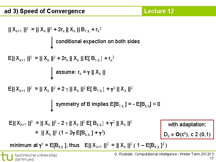
ad 3) Speed of Convergence Lecture 12 || Xk+1 ||2 = || Xk ||2 + 2 rk || Xk || B 1: + rk 2 conditional expection on both sides E|| Xk+1 ||2 = || Xk ||2 + 2 rk || Xk || E[ B 1: ] + rk 2 assume: rk = || Xk || E|| Xk+1 ||2 = || Xk ||2 + 2 || Xk ||2 E[ B 1: ] + 2 || Xk ||2 symmetry of B implies E[B 1: ] = - E[B : ] < 0 E|| Xk+1 ||2 = || Xk ||2 - 2 || Xk ||2 E[ B : ] + 2 || Xk ||2 with adaptation: = || Xk ||2 (1 – 2 E[B : ] + 2) Dk » O(ck), c 2 (0, 1) minimum at * = E[B : ], thus E|| Xk+1 ||2 = || Xk ||2 ( 1 – E[B : ]2 ) G. Rudolph: Computational Intelligence ▪ Winter Term 2012/13 17

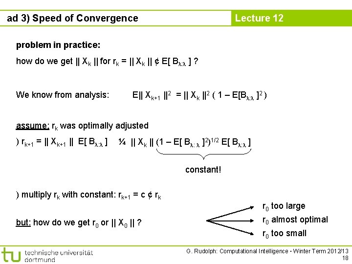
ad 3) Speed of Convergence Lecture 12 problem in practice: how do we get || Xk || for rk = || Xk || ¢ E[ B : ] ? We know from analysis: E|| Xk+1 ||2 = || Xk ||2 ( 1 – E[B : ]2 ) assume: rk was optimally adjusted ) rk+1 = || Xk+1 || E[ B : ] ¼ || Xk || (1 – E[ B : ]2)1/2 E[ B : ] constant! ) multiply rk with constant: rk+1 = c ¢ rk but: how do we get r 0 or || X 0 || ? r 0 too large r 0 almost optimal r 0 too small G. Rudolph: Computational Intelligence ▪ Winter Term 2012/13 18

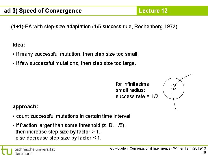
ad 3) Speed of Convergence Lecture 12 (1+1)-EA with step-size adaptation (1/5 success rule, Rechenberg 1973) Idea: • If many successful mutation, then step size too small. • If few successful mutations, then step size too large. for infinitesimal small radius: success rate = 1/2 approach: • count successful mutations in certain time interval • if fraction larger than some threshold (z. B. 1/5), then increase step size by factor > 1, else decrease step size by factor < 1. G. Rudolph: Computational Intelligence ▪ Winter Term 2012/13 19

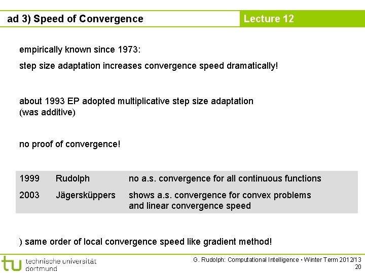
ad 3) Speed of Convergence Lecture 12 empirically known since 1973: step size adaptation increases convergence speed dramatically! about 1993 EP adopted multiplicative step size adaptation (was additive) no proof of convergence! 1999 Rudolph no a. s. convergence for all continuous functions 2003 Jägersküppers shows a. s. convergence for convex problems and linear convergence speed ) same order of local convergence speed like gradient method! G. Rudolph: Computational Intelligence ▪ Winter Term 2012/13 20

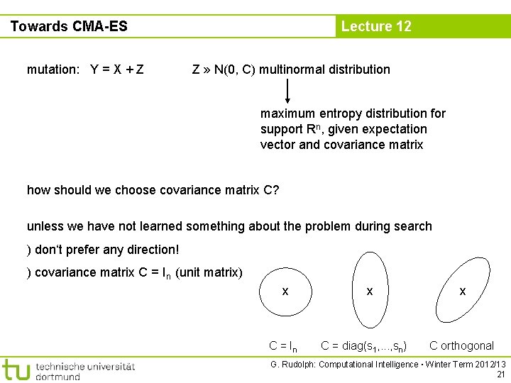
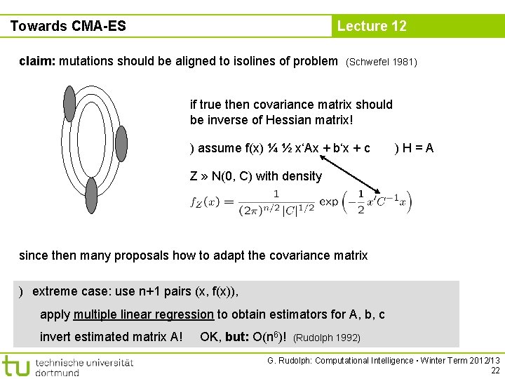
Towards CMA-ES mutation: Y = X + Z Lecture 12 Z » N(0, C) multinormal distribution maximum entropy distribution for support Rn, given expectation vector and covariance matrix how should we choose covariance matrix C? unless we have not learned something about the problem during search ) don‘t prefer any direction! ) covariance matrix C = In (unit matrix) x C = In x C = diag(s 1, . . . , sn) x C orthogonal G. Rudolph: Computational Intelligence ▪ Winter Term 2012/13 21

Towards CMA-ES Lecture 12 claim: mutations should be aligned to isolines of problem (Schwefel 1981) if true then covariance matrix should be inverse of Hessian matrix! ) assume f(x) ¼ ½ x‘Ax + b‘x + c )H=A Z » N(0, C) with density since then many proposals how to adapt the covariance matrix ) extreme case: use n+1 pairs (x, f(x)), apply multiple linear regression to obtain estimators for A, b, c invert estimated matrix A! OK, but: O(n 6)! (Rudolph 1992) G. Rudolph: Computational Intelligence ▪ Winter Term 2012/13 22

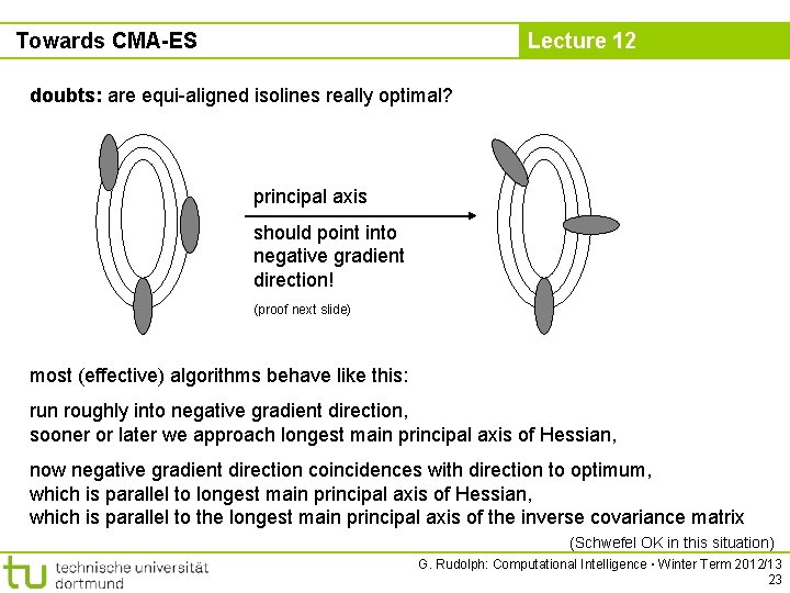
Towards CMA-ES Lecture 12 doubts: are equi-aligned isolines really optimal? principal axis should point into negative gradient direction! (proof next slide) most (effective) algorithms behave like this: run roughly into negative gradient direction, sooner or later we approach longest main principal axis of Hessian, now negative gradient direction coincidences with direction to optimum, which is parallel to longest main principal axis of Hessian, which is parallel to the longest main principal axis of the inverse covariance matrix (Schwefel OK in this situation) G. Rudolph: Computational Intelligence ▪ Winter Term 2012/13 23

Towards CMA-ES Lecture 12 Z = r. Qu, A = B‘B, B = Q-1 if Qu were deterministic. . . ) set Qu = -rf(x) (direction of steepest descent) G. Rudolph: Computational Intelligence ▪ Winter Term 2012/13 24

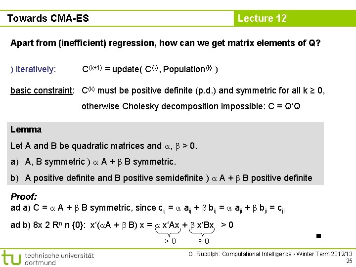
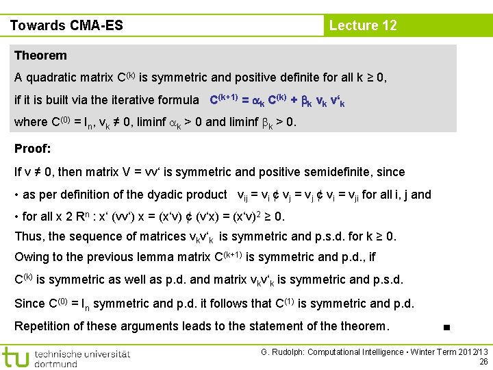
Towards CMA-ES Lecture 12 Apart from (inefficient) regression, how can we get matrix elements of Q? ) iteratively: C(k+1) = update( C(k), Population(k) ) basic constraint: C(k) must be positive definite (p. d. ) and symmetric for all k ≥ 0, otherwise Cholesky decomposition impossible: C = Q‘Q Lemma Let A and B be quadratic matrices and , > 0. a) A, B symmetric ) A + B symmetric. b) A positive definite and B positive semidefinite ) A + B positive definite Proof: ad a) C = A + B symmetric, since cij = aij + bij = aji + bji = cji ad b) 8 x 2 Rn n {0}: x‘( A + B) x = x‘Ax + x‘Bx > 0 >0 ≥ 0 ■ G. Rudolph: Computational Intelligence ▪ Winter Term 2012/13 25

Towards CMA-ES Lecture 12 Theorem A quadratic matrix C(k) is symmetric and positive definite for all k ≥ 0, if it is built via the iterative formula C(k+1) = k C(k) + k vk v‘k where C(0) = In, vk ≠ 0, liminf k > 0 and liminf k > 0. Proof: If v ≠ 0, then matrix V = vv‘ is symmetric and positive semidefinite, since • as per definition of the dyadic product vij = vi ¢ vj = vj ¢ vi = vji for all i, j and • for all x 2 Rn : x‘ (vv‘) x = (x‘v) ¢ (v‘x) = (x‘v)2 ≥ 0. Thus, the sequence of matrices vkv‘k is symmetric and p. s. d. for k ≥ 0. Owing to the previous lemma matrix C(k+1) is symmetric and p. d. , if C(k) is symmetric as well as p. d. and matrix vkv‘k is symmetric and p. s. d. Since C(0) = In symmetric and p. d. it follows that C(1) is symmetric and p. d. Repetition of these arguments leads to the statement of theorem. ■ G. Rudolph: Computational Intelligence ▪ Winter Term 2012/13 26

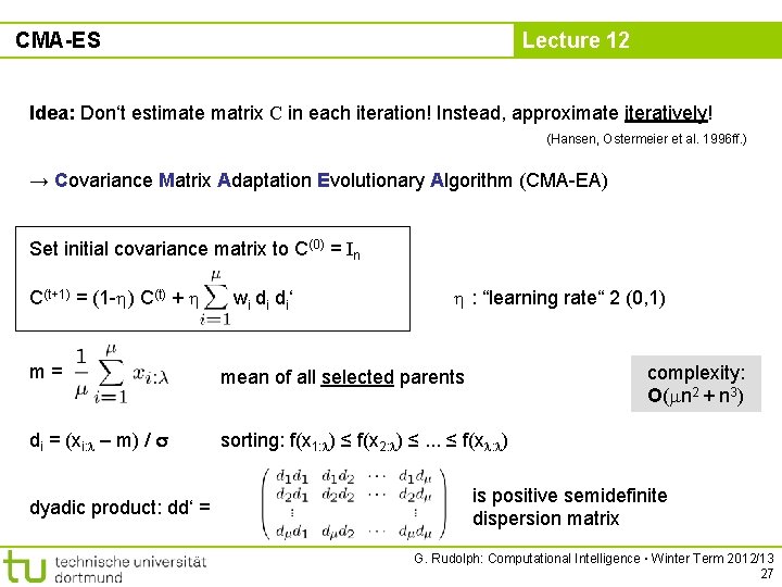
CMA-ES Lecture 12 Idea: Don‘t estimate matrix C in each iteration! Instead, approximate iteratively! (Hansen, Ostermeier et al. 1996 ff. ) → Covariance Matrix Adaptation Evolutionary Algorithm (CMA-EA) Set initial covariance matrix to C(0) = In C(t+1) = (1 - ) C(t) + wi di di‘ : “learning rate“ 2 (0, 1) m= mean of all selected parents di = (xi: – m) / sorting: f(x 1: ) ≤ f(x 2: ) ≤. . . ≤ f(x : ) dyadic product: dd‘ = complexity: O( n 2 + n 3) is positive semidefinite dispersion matrix G. Rudolph: Computational Intelligence ▪ Winter Term 2012/13 27

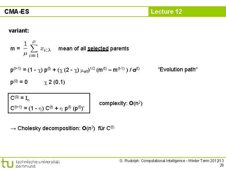
CMA-ES Lecture 12 variant: m= mean of all selected parents p(t+1) = (1 - ) p(t) + ( (2 - ) eff)1/2 (m(t) – m(t-1) ) / (t) p(0) = 0 “Evolution path“ 2 (0, 1) C(0) = In C(t+1) = (1 - ) C(t) + p(t) (p(t))‘ complexity: O(n 2) → Cholesky decomposition: O(n 3) für C(t) G. Rudolph: Computational Intelligence ▪ Winter Term 2012/13 28

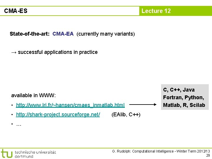
CMA-ES Lecture 12 State-of-the-art: CMA-EA (currently many variants) → successful applications in practice available in WWW: • http: //www. lri. fr/~hansen/cmaes_inmatlab. html • http: //shark-project. sourceforge. net/ C, C++, Java Fortran, Python, Matlab, R, Scilab (EAlib, C++) • … G. Rudolph: Computational Intelligence ▪ Winter Term 2012/13 29