Computational Intelligence Winter Term 201920 Prof Dr Gnter

Computational Intelligence Winter Term 2019/20 Prof. Dr. Günter Rudolph Lehrstuhl für Algorithm Engineering (LS 11) Fakultät für Informatik TU Dortmund

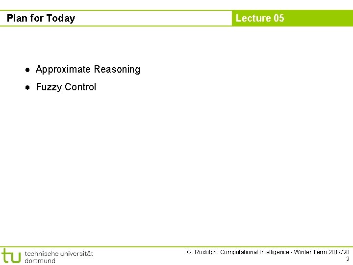
Plan for Today Lecture 05 ● Approximate Reasoning ● Fuzzy Control G. Rudolph: Computational Intelligence ▪ Winter Term 2019/20 2

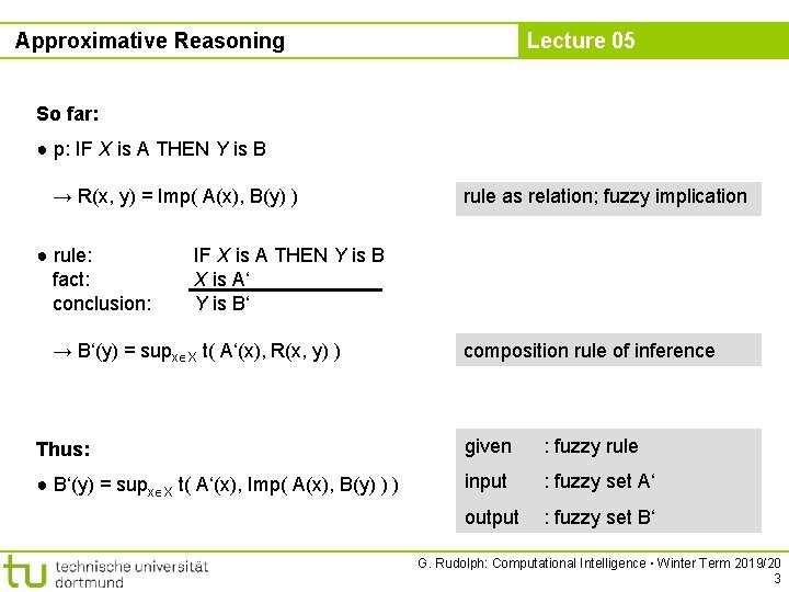
Approximative Reasoning Lecture 05 So far: ● p: IF X is A THEN Y is B → R(x, y) = Imp( A(x), B(y) ) ● rule: fact: conclusion: rule as relation; fuzzy implication IF X is A THEN Y is B X is A‘ Y is B‘ → B‘(y) = supx X t( A‘(x), R(x, y) ) composition rule of inference Thus: given : fuzzy rule ● B‘(y) = supx X t( A‘(x), Imp( A(x), B(y) ) ) input : fuzzy set A‘ output : fuzzy set B‘ G. Rudolph: Computational Intelligence ▪ Winter Term 2019/20 3

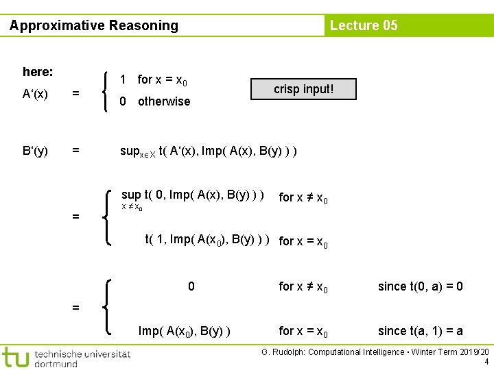
Approximative Reasoning here: A‘(x) = B‘(y) = Lecture 05 1 for x = x 0 crisp input! 0 otherwise supx X t( A‘(x), Imp( A(x), B(y) ) ) sup t( 0, Imp( A(x), B(y) ) ) = x ≠ x 0 for x ≠ x 0 t( 1, Imp( A(x 0), B(y) ) ) for x = x 0 0 for x ≠ x 0 since t(0, a) = 0 for x = x 0 since t(a, 1) = a = Imp( A(x 0), B(y) ) G. Rudolph: Computational Intelligence ▪ Winter Term 2019/20 4

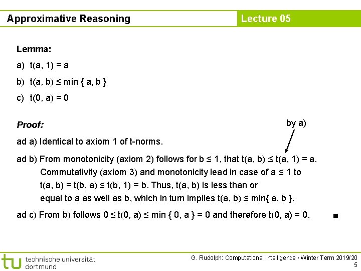
Approximative Reasoning Lecture 05 Lemma: a) t(a, 1) = a b) t(a, b) ≤ min { a, b } c) t(0, a) = 0 Proof: by a) ad a) Identical to axiom 1 of t-norms. ad b) From monotonicity (axiom 2) follows for b ≤ 1, that t(a, b) ≤ t(a, 1) = a. Commutativity (axiom 3) and monotonicity lead in case of a ≤ 1 to t(a, b) = t(b, a) ≤ t(b, 1) = b. Thus, t(a, b) is less than or equal to a as well as b, which in turn implies t(a, b) ≤ min{ a, b }. ad c) From b) follows 0 ≤ t(0, a) ≤ min { 0, a } = 0 and therefore t(0, a) = 0. ■ G. Rudolph: Computational Intelligence ▪ Winter Term 2019/20 5

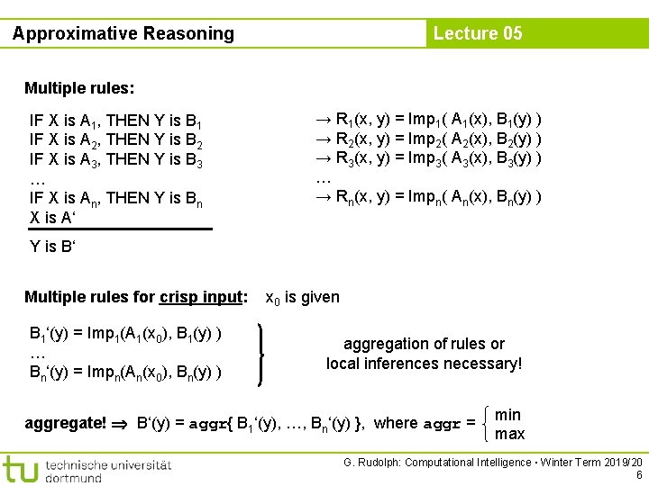
Approximative Reasoning Lecture 05 Multiple rules: IF X is A 1, THEN Y is B 1 IF X is A 2, THEN Y is B 2 IF X is A 3, THEN Y is B 3 … IF X is An, THEN Y is Bn X is A‘ → R 1(x, y) = Imp 1( A 1(x), B 1(y) ) → R 2(x, y) = Imp 2( A 2(x), B 2(y) ) → R 3(x, y) = Imp 3( A 3(x), B 3(y) ) … → Rn(x, y) = Impn( An(x), Bn(y) ) Y is B‘ Multiple rules for crisp input: B 1‘(y) = Imp 1(A 1(x 0), B 1(y) ) … Bn‘(y) = Impn(An(x 0), Bn(y) ) x 0 is given aggregation of rules or local inferences necessary! aggregate! B‘(y) = aggr{ B 1‘(y), …, Bn‘(y) }, where aggr = min max G. Rudolph: Computational Intelligence ▪ Winter Term 2019/20 6

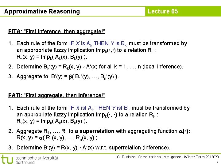
Approximative Reasoning Lecture 05 FITA: “First inference, then aggregate!“ 1. Each rule of the form IF X is Ak THEN Y is Bk must be transformed by an appropriate fuzzy implication Impk(·, ·) to a relation Rk : Rk(x, y) = Impk( Ak(x), Bk(y) ). 2. Determine Bk‘(y) = Rk(x, y) ◦ A‘(x) for all k = 1, …, n (local inference). 3. Aggregate to B‘(y) = ( B 1‘(y), …, Bn‘(y) ). FATI: “First aggregate, then inference!“ 1. Each rule of the form IF X ist Ak THEN Y ist Bk must be transformed by an appropriate fuzzy implication Impk(·, ·) to a relation Rk : Rk(x, y) = Impk( Ak(x), Bk(y) ). 2. Aggregate R 1, …, Rn to a superrelation with aggregating function (·): R(x, y) = ( R 1(x, y), …, Rn(x, y) ). 3. Determine B‘(y) = R(x, y) ◦ A‘(x) w. r. t. superrelation (inference). G. Rudolph: Computational Intelligence ▪ Winter Term 2019/20 7

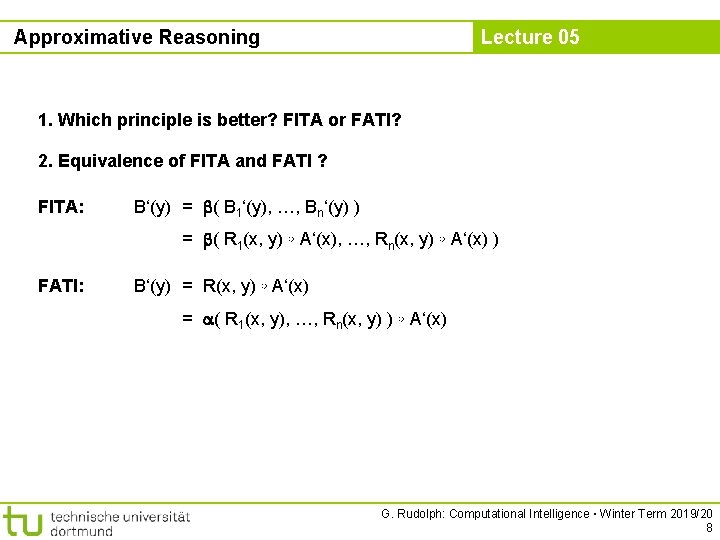
Approximative Reasoning Lecture 05 1. Which principle is better? FITA or FATI? 2. Equivalence of FITA and FATI ? FITA: B‘(y) = ( B 1‘(y), …, Bn‘(y) ) = ( R 1(x, y) ◦ A‘(x), …, Rn(x, y) ◦ A‘(x) ) FATI: B‘(y) = R(x, y) ◦ A‘(x) = ( R 1(x, y), …, Rn(x, y) ) ◦ A‘(x) G. Rudolph: Computational Intelligence ▪ Winter Term 2019/20 8

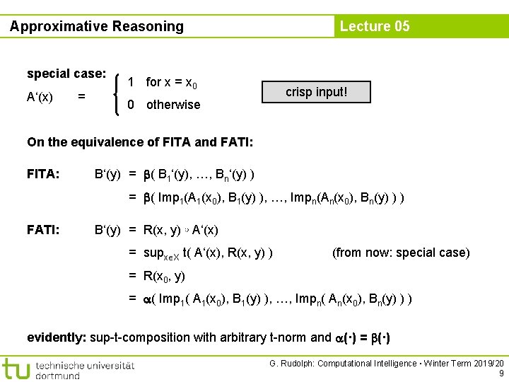
Approximative Reasoning special case: A‘(x) = Lecture 05 1 for x = x 0 crisp input! 0 otherwise On the equivalence of FITA and FATI: FITA: B‘(y) = ( B 1‘(y), …, Bn‘(y) ) = ( Imp 1(A 1(x 0), B 1(y) ), …, Impn(An(x 0), Bn(y) ) ) FATI: B‘(y) = R(x, y) ◦ A‘(x) = supx X t( A‘(x), R(x, y) ) (from now: special case) = R(x 0, y) = ( Imp 1( A 1(x 0), B 1(y) ), …, Impn( An(x 0), Bn(y) ) ) evidently: sup-t-composition with arbitrary t-norm and (·) = (·) G. Rudolph: Computational Intelligence ▪ Winter Term 2019/20 9

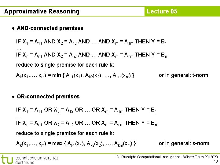
Approximative Reasoning Lecture 05 ● AND-connected premises IF X 1 = A 11 AND X 2 = A 12 AND … AND Xm = A 1 m THEN Y = B 1 … IF Xn = An 1 AND X 2 = An 2 AND … AND Xm = Anm THEN Y = Bn reduce to single premise for each rule k: Ak(x 1, …, xm) = min { Ak 1(x 1), Ak 2(x 2), …, Akm(xm) } or in general: t-norm ● OR-connected premises IF X 1 = A 11 OR X 2 = A 12 OR … OR Xm = A 1 m THEN Y = B 1 … IF Xn = An 1 OR X 2 = An 2 OR … OR Xm = Anm THEN Y = Bn reduce to single premise for each rule k: Ak(x 1, …, xm) = max { Ak 1(x 1), Ak 2(x 2), …, Akm(xm) } or in general: s-norm G. Rudolph: Computational Intelligence ▪ Winter Term 2019/20 10

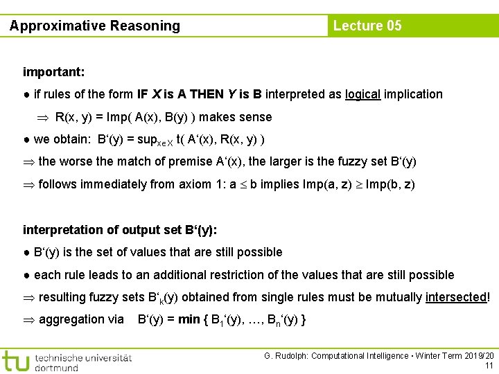
Approximative Reasoning Lecture 05 important: ● if rules of the form IF X is A THEN Y is B interpreted as logical implication R(x, y) = Imp( A(x), B(y) ) makes sense ● we obtain: B‘(y) = supx X t( A‘(x), R(x, y) ) the worse the match of premise A‘(x), the larger is the fuzzy set B‘(y) follows immediately from axiom 1: a b implies Imp(a, z) Imp(b, z) interpretation of output set B‘(y): ● B‘(y) is the set of values that are still possible ● each rule leads to an additional restriction of the values that are still possible resulting fuzzy sets B‘k(y) obtained from single rules must be mutually intersected! aggregation via B‘(y) = min { B 1‘(y), …, Bn‘(y) } G. Rudolph: Computational Intelligence ▪ Winter Term 2019/20 11

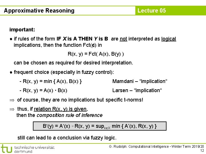
Approximative Reasoning Lecture 05 important: ● if rules of the form IF X is A THEN Y is B are not interpreted as logical implications, then the function Fct(¢) in R(x, y) = Fct( A(x), B(y) ) can be chosen as required for desired interpretation. ● frequent choice (especially in fuzzy control): - R(x, y) = min { A(x), B(x) } Mamdani – “implication“ - R(x, y) = A(x) · B(x) Larsen – “implication“ of course, they are no implications but specific t-norms! thus, if relation R(x, y) is given, then the composition rule of inference B‘(y) = A‘(x) ◦ R(x, y) = supx X min { A’(x), R(x, y) } still can lead to a conclusion via fuzzy logic. G. Rudolph: Computational Intelligence ▪ Winter Term 2019/20 12

Approximative Reasoning example: Lecture 05 [JM 96, S. 244 ff. ] industrial drill machine → control of cooling supply modellinguistic variable : rotation speed linguistic terms : very low, medium, high, very high ground set : X with 0 ≤ x ≤ 18000 [rpm] 1 vl 1000 l 5000 m 9000 h 13000 vh 17000 rotation speed G. Rudolph: Computational Intelligence ▪ Winter Term 2019/20 13

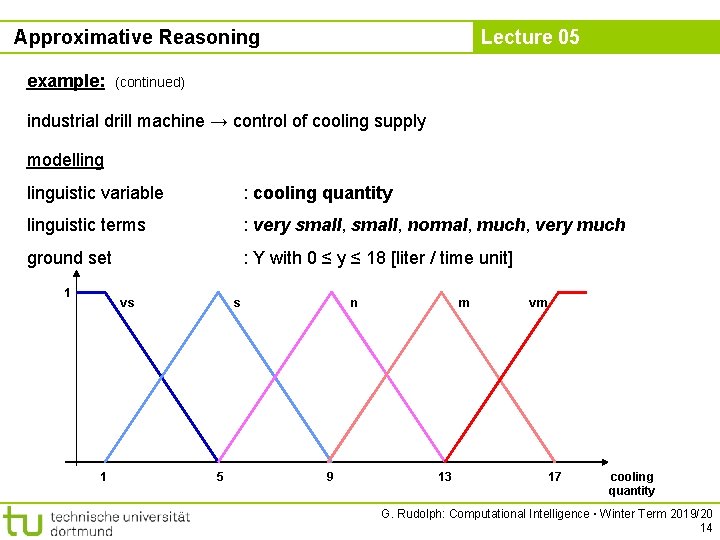
Approximative Reasoning example: Lecture 05 (continued) industrial drill machine → control of cooling supply modellinguistic variable : cooling quantity linguistic terms : very small, normal, much, very much ground set : Y with 0 ≤ y ≤ 18 [liter / time unit] 1 vs 1 s 5 n 9 m 13 vm 17 cooling quantity G. Rudolph: Computational Intelligence ▪ Winter Term 2019/20 14

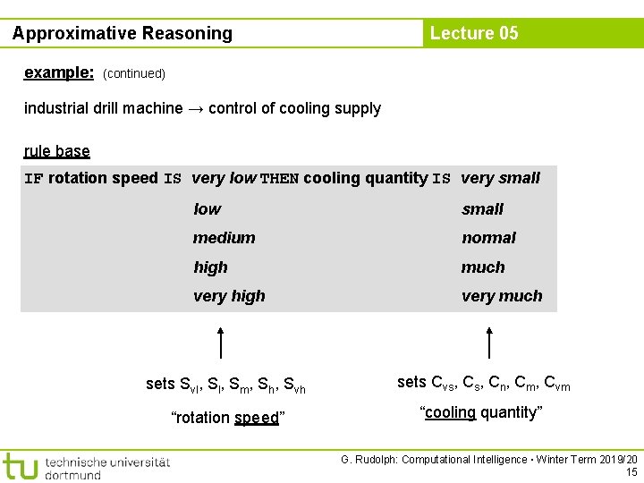
Approximative Reasoning example: Lecture 05 (continued) industrial drill machine → control of cooling supply rule base IF rotation speed IS very low THEN cooling quantity IS very small low small medium normal high much very high very much sets Svl, Sm, Sh, Svh sets Cvs, Cn, Cm, Cvm “rotation speed” “cooling quantity” G. Rudolph: Computational Intelligence ▪ Winter Term 2019/20 15

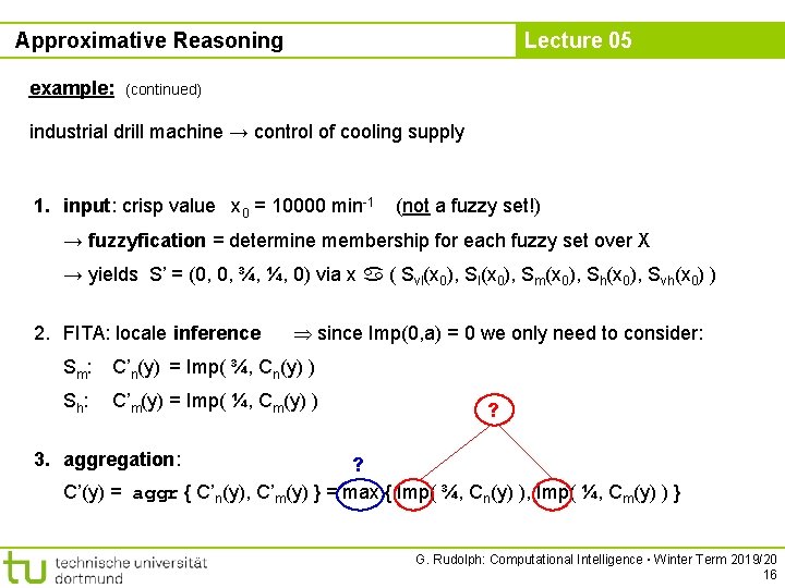
Approximative Reasoning example: Lecture 05 (continued) industrial drill machine → control of cooling supply 1. input: crisp value x 0 = 10000 min-1 (not a fuzzy set!) → fuzzyfication = determine membership for each fuzzy set over X → yields S’ = (0, 0, ¾, ¼, 0) via x ( Svl(x 0), Sm(x 0), Sh(x 0), Svh(x 0) ) 2. FITA: locale inference since Imp(0, a) = 0 we only need to consider: Sm: C’n(y) = Imp( ¾, Cn(y) ) Sh: C’m(y) = Imp( ¼, Cm(y) ) ? 3. aggregation: ? C’(y) = aggr { C’n(y), C’m(y) } = max { Imp( ¾, Cn(y) ), Imp( ¼, Cm(y) ) } G. Rudolph: Computational Intelligence ▪ Winter Term 2019/20 16

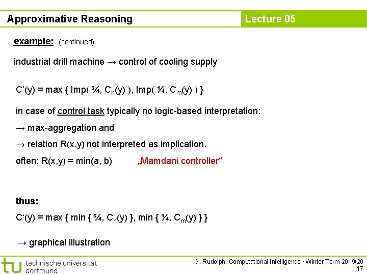
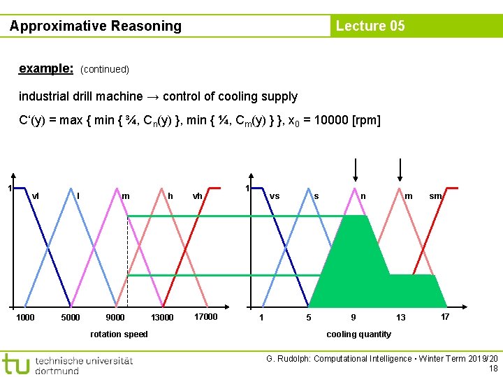
Approximative Reasoning example: Lecture 05 (continued) industrial drill machine → control of cooling supply C’(y) = max { Imp( ¾, Cn(y) ), Imp( ¼, Cm(y) ) } in case of control task typically no logic-based interpretation: → max-aggregation and → relation R(x, y) not interpreted as implication. often: R(x, y) = min(a, b) „Mamdani controller“ thus: C‘(y) = max { min { ¾, Cn(y) }, min { ¼, Cm(y) } } → graphical illustration G. Rudolph: Computational Intelligence ▪ Winter Term 2019/20 17

Approximative Reasoning example: Lecture 05 (continued) industrial drill machine → control of cooling supply C‘(y) = max { min { ¾, Cn(y) }, min { ¼, Cm(y) } }, x 0 = 10000 [rpm] 1 vl 1000 l 5000 m 9000 rotation speed h 13000 vh 17000 1 vs 1 s 5 n 9 m 13 sm 17 cooling quantity G. Rudolph: Computational Intelligence ▪ Winter Term 2019/20 18

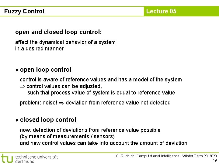
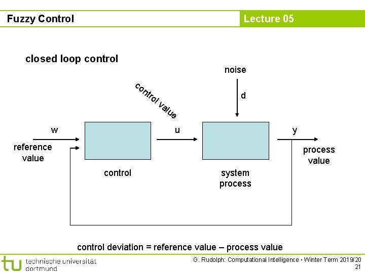
Fuzzy Control Lecture 05 open and closed loop control: affect the dynamical behavior of a system in a desired manner ● open loop control is aware of reference values and has a model of the system control values can be adjusted, such that process value of system is equal to reference value problem: noise! deviation from reference value not detected ● closed loop control now: detection of deviations from reference value possible (by means of measurements / sensors) and new control values can take into account the amount of deviation G. Rudolph: Computational Intelligence ▪ Winter Term 2019/20 19

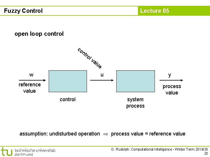
Fuzzy Control Lecture 05 open loop control co nt w ro lv alu e u y reference value process value control system process assumption: undisturbed operation process value = reference value G. Rudolph: Computational Intelligence ▪ Winter Term 2019/20 20

Fuzzy Control Lecture 05 closed loop control noise co nt w ro d lv alu e u y reference value process value control system process control deviation = reference value – process value G. Rudolph: Computational Intelligence ▪ Winter Term 2019/20 21

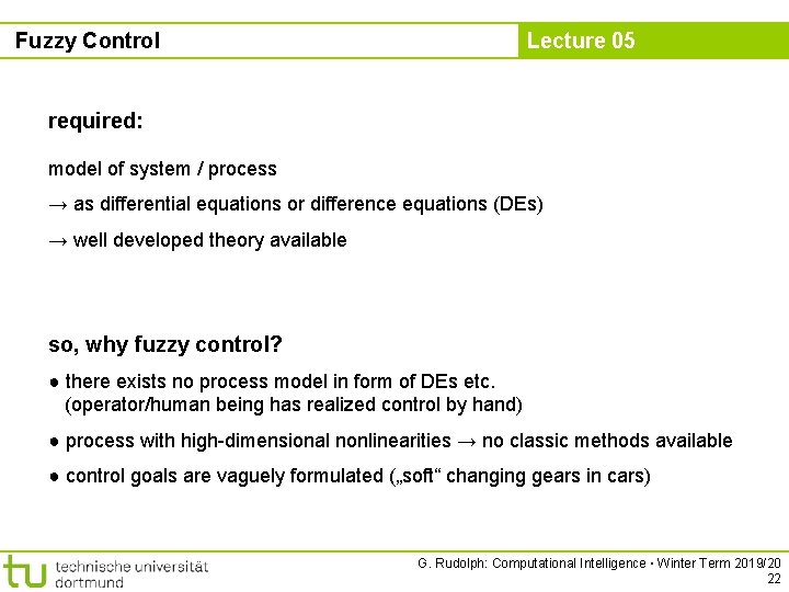
Fuzzy Control Lecture 05 required: model of system / process → as differential equations or difference equations (DEs) → well developed theory available so, why fuzzy control? ● there exists no process model in form of DEs etc. (operator/human being has realized control by hand) ● process with high-dimensional nonlinearities → no classic methods available ● control goals are vaguely formulated („soft“ changing gears in cars) G. Rudolph: Computational Intelligence ▪ Winter Term 2019/20 22

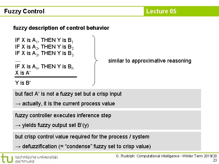
Fuzzy Control Lecture 05 fuzzy description of control behavior IF X is A 1, THEN Y is B 1 IF X is A 2, THEN Y is B 2 IF X is A 3, THEN Y is B 3 … IF X is An, THEN Y is Bn X is A‘ similar to approximative reasoning Y is B‘ but fact A‘ is not a fuzzy set but a crisp input → actually, it is the current process value fuzzy controller executes inference step → yields fuzzy output set B‘(y) but crisp control value required for the process / system → defuzzification (= “condense” fuzzy set to crisp value) G. Rudolph: Computational Intelligence ▪ Winter Term 2019/20 23

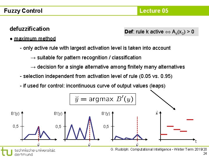
Fuzzy Control Lecture 05 defuzzification Def: rule k active Ak(x 0) > 0 ● maximum method - only active rule with largest activation level is taken into account → suitable for pattern recognition / classification → decision for a single alternative among finitely many alternatives - selection independent from activation level of rule (0. 05 vs. 0. 95) - if used for control: incontinuous curve of output values (leaps) B‘(y) 0, 5 t G. Rudolph: Computational Intelligence ▪ Winter Term 2019/20 24

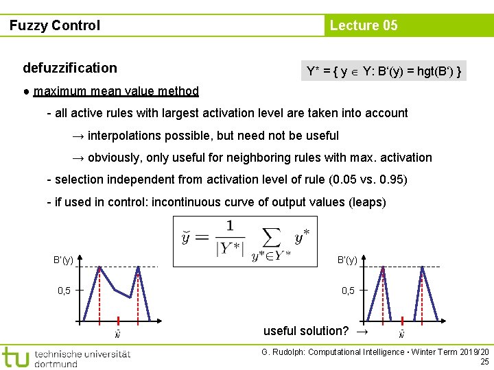
Fuzzy Control defuzzification Lecture 05 Y* = { y Y: B‘(y) = hgt(B‘) } ● maximum mean value method - all active rules with largest activation level are taken into account → interpolations possible, but need not be useful → obviously, only useful for neighboring rules with max. activation - selection independent from activation level of rule (0. 05 vs. 0. 95) - if used in control: incontinuous curve of output values (leaps) B‘(y) 0, 5 useful solution? → G. Rudolph: Computational Intelligence ▪ Winter Term 2019/20 25

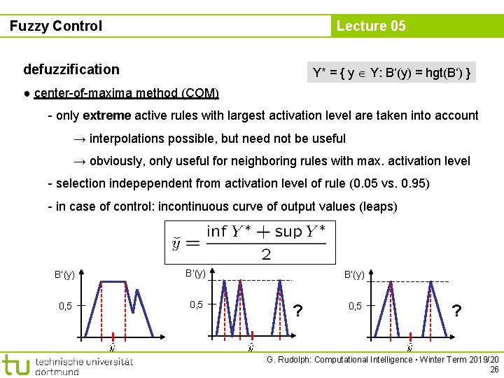
Fuzzy Control Lecture 05 defuzzification Y* = { y Y: B‘(y) = hgt(B‘) } ● center-of-maxima method (COM) - only extreme active rules with largest activation level are taken into account → interpolations possible, but need not be useful → obviously, only useful for neighboring rules with max. activation level - selection indepependent from activation level of rule (0. 05 vs. 0. 95) - in case of control: incontinuous curve of output values (leaps) B‘(y) 0, 5 B‘(y) ? 0, 5 ? G. Rudolph: Computational Intelligence ▪ Winter Term 2019/20 26

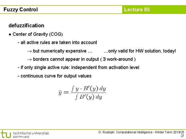
Fuzzy Control Lecture 05 defuzzification ● Center of Gravity (COG) - all active rules are taken into account → but numerically expensive … …only valid for HW solution, today! → borders cannot appear in output ( work-around ) - if only single active rule: independent from activation level - continuous curve for output values G. Rudolph: Computational Intelligence ▪ Winter Term 2019/20 27

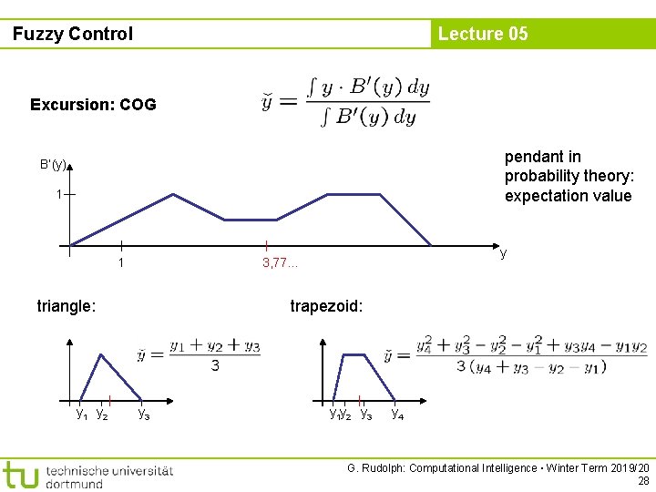
Fuzzy Control Lecture 05 Excursion: COG pendant in probability theory: expectation value B‘(y) 1 1 triangle: y 1 y 2 y 3, 77. . . trapezoid: y 3 y 1 y 2 y 3 y 4 G. Rudolph: Computational Intelligence ▪ Winter Term 2019/20 28

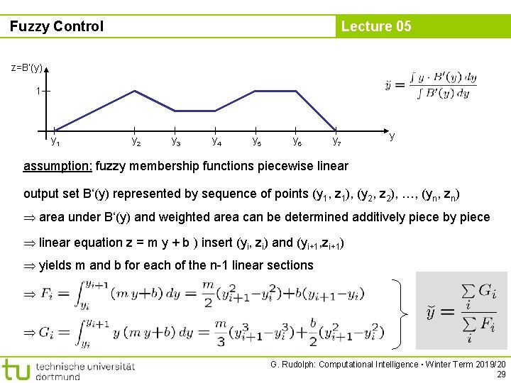
Fuzzy Control Lecture 05 z=B‘(y) 1 y 2 y 3 y 4 y 5 y 6 y 7 y assumption: fuzzy membership functions piecewise linear output set B‘(y) represented by sequence of points (y 1, z 1), (y 2, z 2), …, (yn, zn) area under B‘(y) and weighted area can be determined additively piece by piece linear equation z = m y + b ) insert (yi, zi) and (yi+1, zi+1) yields m and b for each of the n-1 linear sections G. Rudolph: Computational Intelligence ▪ Winter Term 2019/20 29

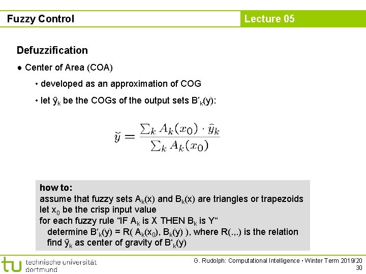
Fuzzy Control Lecture 05 Defuzzification ● Center of Area (COA) • developed as an approximation of COG • let ŷk be the COGs of the output sets B’k(y): how to: assume that fuzzy sets Ak(x) and Bk(x) are triangles or trapezoids let x 0 be the crisp input value for each fuzzy rule “IF Ak is X THEN Bk is Y“ determine B‘k(y) = R( Ak(x 0), Bk(y) ), where R(. , . ) is the relation find ŷk as center of gravity of B‘k(y) G. Rudolph: Computational Intelligence ▪ Winter Term 2019/20 30