Coherent Measures of Risk David Heath Carnegie Mellon

Coherent Measures of Risk David Heath Carnegie Mellon University Joint work with Philippe Artzner, Freddy Delbaen, Jean-Marc Eber; research partially funded by Société Generale

Measuring Risk u Purpose: – Manage and control risk – Make good risk/return tradeoff – “Risk adjust” traders’ profits u To help with: – Regulation of traders and banks – Portfolio selection – Motivating traders to reduce risk

How should a risk measure behave? u Should provide a basis for setting “capital requirements” u Should be “reasonable” – Encourage diversification – Should respect “more is better” u Should be useable as a management tool – Should be compatible with allocation of risk limits to desks – Should provide sensible way to “risk-adjust” gains of different investment strategies (desks)

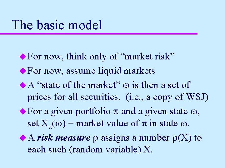
The basic model u For now, think only of “market risk” u For now, assume liquid markets u A “state of the market” w is then a set of prices for all securities. (i. e. , a copy of WSJ) u For a given portfolio p and a given state w, set Xp(w) = market value of p in state w. u A risk measure r assigns a number r(X) to each such (random variable) X.

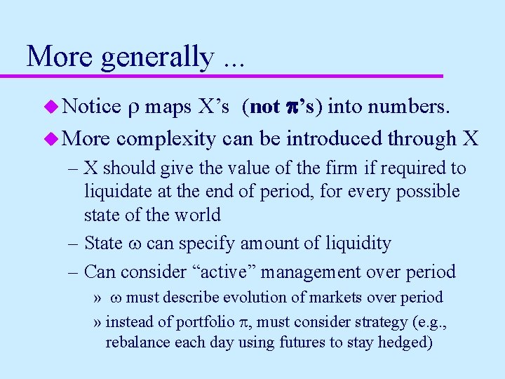
More generally. . . r maps X’s (not p’s) into numbers. u More complexity can be introduced through X u Notice – X should give the value of the firm if required to liquidate at the end of period, for every possible state of the world – State w can specify amount of liquidity – Can consider “active” management over period » w must describe evolution of markets over period » instead of portfolio p, must consider strategy (e. g. , rebalance each day using futures to stay hedged)

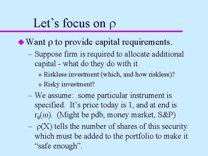
Let’s focus on r u Want r to provide capital requirements. – Suppose firm is required to allocate additional capital - what do they do with it » Riskless investment (which, and how riskless)? » Risky investment? – We assume: some particular instrument is specified. It’s price today is 1, and at end is r 0(w). (Might be pdb, money market, S&P) – r(X) tells the number of shares of this security which must be added to the portfolio to make it “safe enough”.

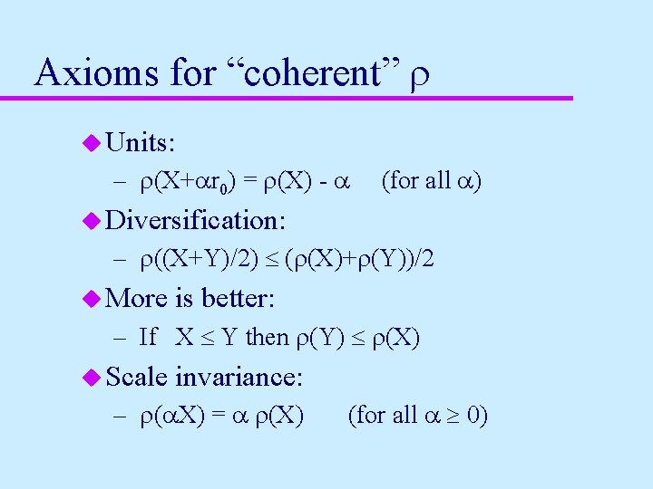
Axioms for “coherent” r u Units: – r(X+ar 0) = r(X) - a (for all a) u Diversification: – r((X+Y)/2) £ (r(X)+r(Y))/2 u More is better: – If X £ Y then r(Y) £ r(X) u Scale invariance: – r(a. X) = a r(X) (for all a ³ 0)

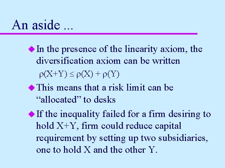
An aside. . . u In the presence of the linearity axiom, the diversification axiom can be written r(X+Y) £ r(X) + r(Y) u This means that a risk limit can be “allocated” to desks u If the inequality failed for a firm desiring to hold X+Y, firm could reduce capital requirement by setting up two subsidiaries, one to hold X and the other Y.

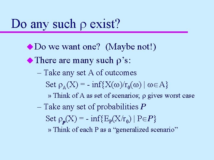
Do any such r exist? u Do we want one? (Maybe not!) u There are many such r’s: – Take any set A of outcomes Set r. A(X) = - inf{X(w)/r 0(w) | wÎA} » Think of A as set of scenarios; r gives worst case – Take any set of probabilities P Set rp(X) = - inf{EP(X/r 0) | PÎP} » Think of each P as a “generalized scenario”

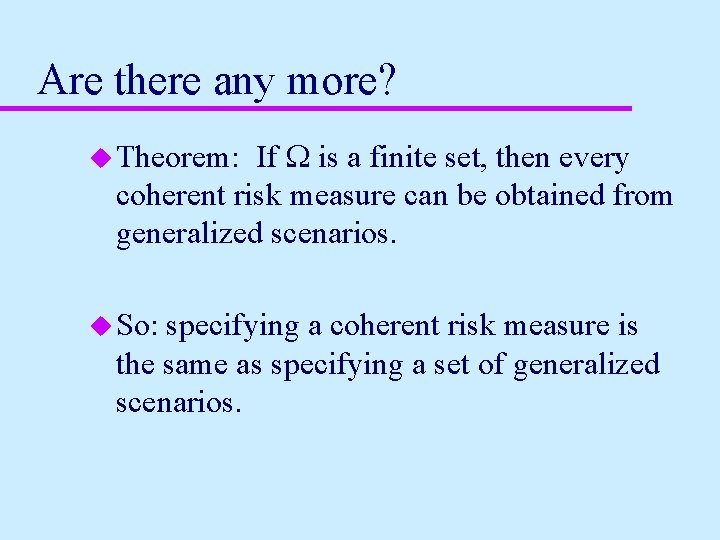
Are there any more? If W is a finite set, then every coherent risk measure can be obtained from generalized scenarios. u Theorem: u So: specifying a coherent risk measure is the same as specifying a set of generalized scenarios.

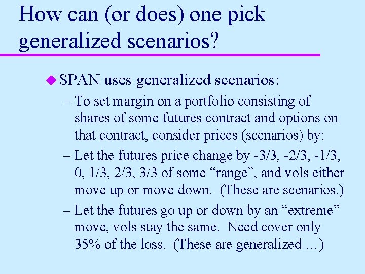
How can (or does) one pick generalized scenarios? u SPAN uses generalized scenarios: – To set margin on a portfolio consisting of shares of some futures contract and options on that contract, consider prices (scenarios) by: – Let the futures price change by -3/3, -2/3, -1/3, 0, 1/3, 2/3, 3/3 of some “range”, and vols either move up or move down. (These are scenarios. ) – Let the futures go up or down by an “extreme” move, vols stay the same. Need cover only 35% of the loss. (These are generalized …)

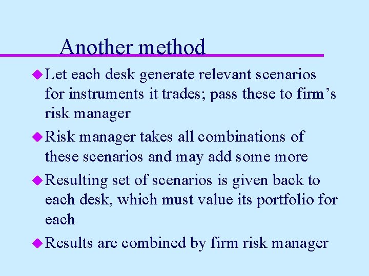
Another method u Let each desk generate relevant scenarios for instruments it trades; pass these to firm’s risk manager u Risk manager takes all combinations of these scenarios and may add some more u Resulting set of scenarios is given back to each desk, which must value its portfolio for each u Results are combined by firm risk manager

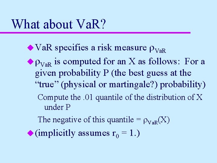
What about Va. R? specifies a risk measure r. Va. R u r. Va. R is computed for an X as follows: For a given probability P (the best guess at the “true” (physical or martingale? ) probability) u Va. R Compute the. 01 quantile of the distribution of X under P The negative of this quantile = r. Va. R(X) u (implicitly assumes r 0 = 1. )

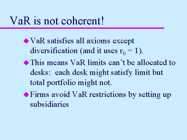
Va. R is not coherent! u Va. R satisfies all axioms except diversification (and it uses r 0 = 1). u This means Va. R limits can’t be allocated to desks: each desk might satisfy limit but total portfolio might not. u Firms avoid Va. R restrictions by setting up subsidiaries

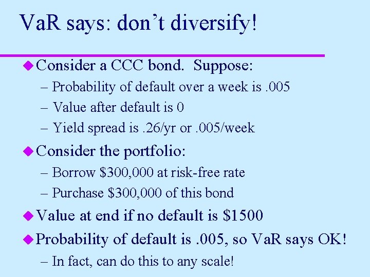
Va. R says: don’t diversify! u Consider a CCC bond. Suppose: – Probability of default over a week is. 005 – Value after default is 0 – Yield spread is. 26/yr or. 005/week u Consider the portfolio: – Borrow $300, 000 at risk-free rate – Purchase $300, 000 of this bond u Value at end if no default is $1500 u Probability of default is. 005, so Va. R says OK! – In fact, can do this to any scale!

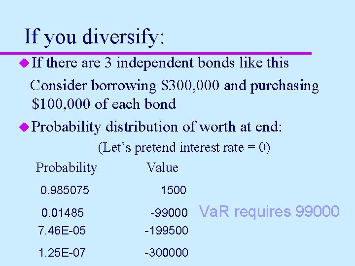
If you diversify: u If there are 3 independent bonds like this Consider borrowing $300, 000 and purchasing $100, 000 of each bond u Probability distribution of worth at end: (Let’s pretend interest rate = 0) Probability Value 0. 985075 1500 0. 01485 -99000 7. 46 E-05 -199500 1. 25 E-07 -300000 Va. R requires 99000

Even scarier u Most firms want to “get the highest return per unit of risk. ” u If they use Va. R to measure risk, they’ll be led to pile up the losses on a “small” set of scenarios (a set with probability less than. 01) u If they use “black box” approach to reducing Va. R they’ll do the same, probably without realizing it!

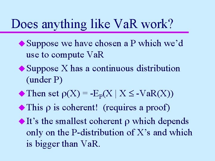
Does anything like Va. R work? u Suppose we have chosen a P which we’d use to compute Va. R u Suppose X has a continuous distribution (under P) u Then set r(X) = -EP(X | X £ -Va. R(X)) u This r is coherent! (requires a proof) u It’s the smallest coherent r which depends only on the P-distribution of X’s and which is bigger than Va. R.

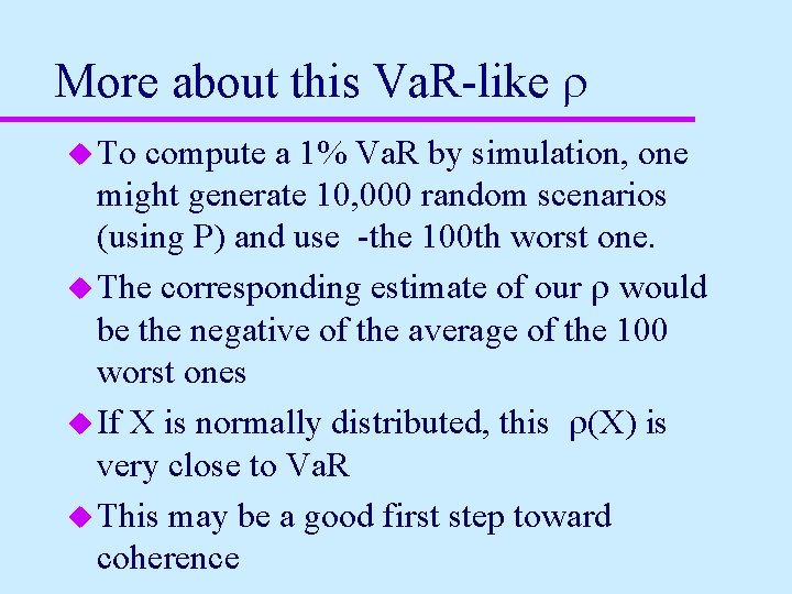
More about this Va. R-like r u To compute a 1% Va. R by simulation, one might generate 10, 000 random scenarios (using P) and use -the 100 th worst one. u The corresponding estimate of our r would be the negative of the average of the 100 worst ones u If X is normally distributed, this r(X) is very close to Va. R u This may be a good first step toward coherence

What’s next? u What are the consequences of trying to maximize return per unit of risk when using a coherent risk measure? – We think that something like that does make sense u Could a bank perform well if each desk used such a measure? – We think so.

Conclusions (to part 1 of talk) u Good risk management requires the use of coherent risk measures u Va. R is not a coherent risk measure – Can induce firms to arrange portfolio so that when the fail, they fail big – Discourages diversification u There is a substitute for Va. R which is more conservative than Va. R, is about as easy to compute, and is coherent

Ongoing research (results tentative!!) u Can coherent risk measures be used for – Firm-wide risk management? – In portfolio selection? u What criteria make one coherent risk measure (or one set of generalized scenarios) better than another? u Can such measures help with – Decentralized portfolio optimization? – “Risk adjusting” trading profits?

Maxing expected return per unit risk u Using Va. R, problem is: – Maximize E(X) – subject to Va. R(X) £ K u Problem is (usually) unbounded – It is if there’s any X with E(X)>0 and Va. R(X) £ 0 (like being short a far out-ofthe-money put) u Va. R constraint is satisfied for arbitrarily large position size!

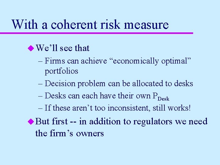
With a coherent risk measure u We’ll see that – Firms can achieve “economically optimal” portfolios – Decision problem can be allocated to desks – Desks can each have their own PDesk – If these aren’t too inconsistent, still works! u But first -- in addition to regulators we need the firm’s owners

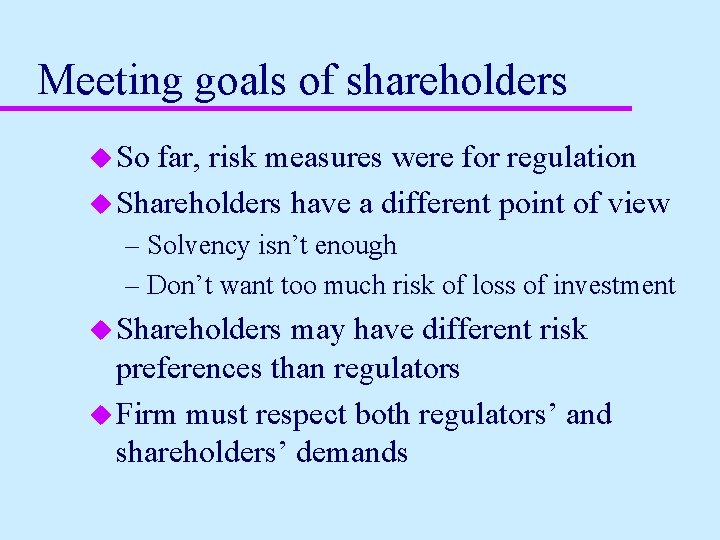
Meeting goals of shareholders u So far, risk measures were for regulation u Shareholders have a different point of view – Solvency isn’t enough – Don’t want too much risk of loss of investment u Shareholders may have different risk preferences than regulators u Firm must respect both regulators’ and shareholders’ demands

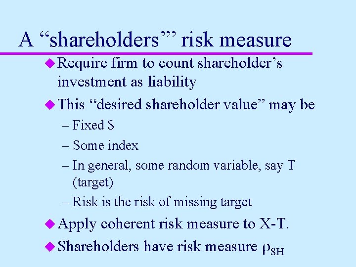
A “shareholders’” risk measure u Require firm to count shareholder’s investment as liability u This “desired shareholder value” may be – Fixed $ – Some index – In general, some random variable, say T (target) – Risk is the risk of missing target u Apply coherent risk measure to X-T. u Shareholders have risk measure r. SH

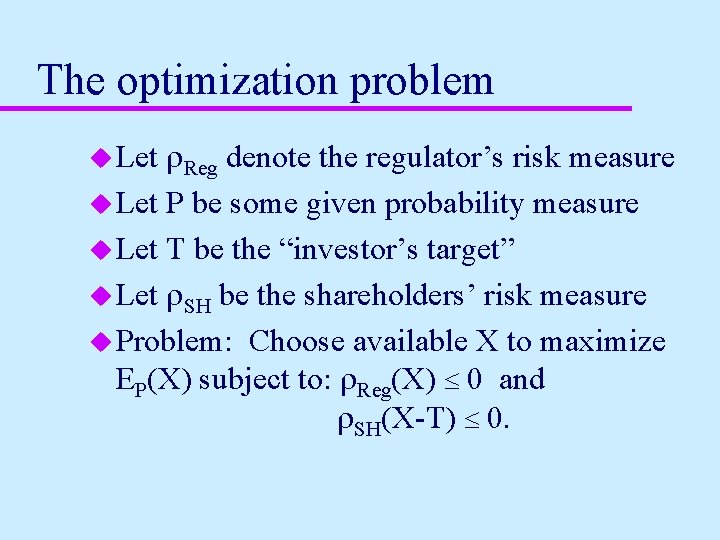
The optimization problem r. Reg denote the regulator’s risk measure u Let P be some given probability measure u Let T be the “investor’s target” u Let r. SH be the shareholders’ risk measure u Problem: Choose available X to maximize EP(X) subject to: r. Reg(X) £ 0 and r. SH(X-T) £ 0. u Let

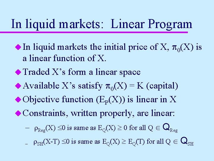
In liquid markets: Linear Program liquid markets the initial price of X, p 0(X) is a linear function of X. u Traded X’s form a linear space u Available X’s satisfy p 0(X) = K (capital) u Objective function (EP(X)) is linear in X u Constraints, written properly, are linear: – r. Reg(X) £ 0 is same as EQ(X) ³ 0 for all Q Î QReg – r. SH(X-T) £ 0 is same as EQ(X) ³ EQ(T) for all Q Î QSH u In

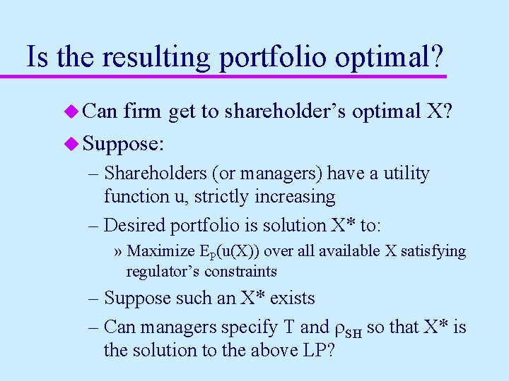
Is the resulting portfolio optimal? u Can firm get to shareholder’s optimal X? u Suppose: – Shareholders (or managers) have a utility function u, strictly increasing – Desired portfolio is solution X* to: » Maximize EP(u(X)) over all available X satisfying regulator’s constraints – Suppose such an X* exists – Can managers specify T and r. SH so that X* is the solution to the above LP?

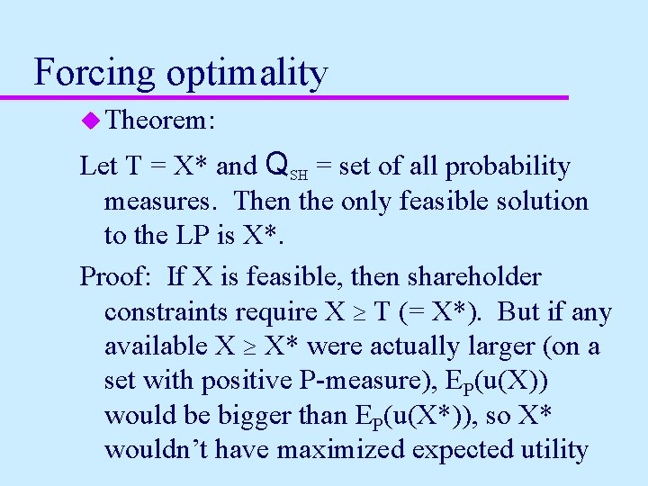
Forcing optimality u Theorem: Let T = X* and QSH = set of all probability measures. Then the only feasible solution to the LP is X*. Proof: If X is feasible, then shareholder constraints require X ³ T (= X*). But if any available X ³ X* were actually larger (on a set with positive P-measure), EP(u(X)) would be bigger than EP(u(X*)), so X* wouldn’t have maximized expected utility

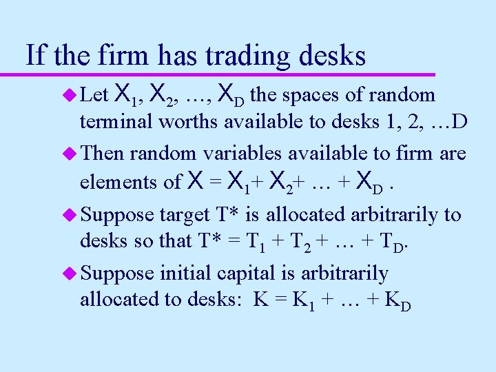
If the firm has trading desks u Let X 1, X 2, …, XD the spaces of random terminal worths available to desks 1, 2, …D u Then random variables available to firm are elements of X = X 1+ X 2+ … + XD. u Suppose target T* is allocated arbitrarily to desks so that T* = T 1 + T 2 + … + TD. u Suppose initial capital is arbitrarily allocated to desks: K = K 1 + … + KD

u and Regulator’s risk is assigned (for each regulator probability Q Î QReg) to desks: r. Q, 1, r. Q, 2, …, r. Q, D summing to 0.

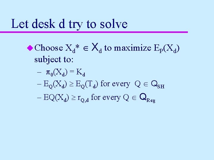
Let desk d try to solve Xd* Î Xd to maximize EP(Xd) subject to: u Choose – p 0(Xd) = Kd – EQ(Xd) ³ EQ(Td) for every Q Î QSH – EQ(Xd) ³ r. Q, d for every Q Î QReg

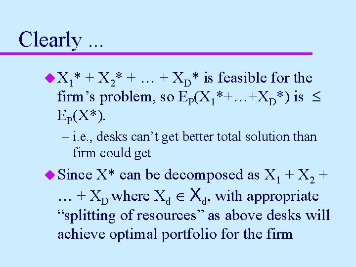
Clearly. . . u X 1* + X 2* + … + XD* is feasible for the firm’s problem, so EP(X 1*+…+XD*) is £ EP(X*). – i. e. , desks can’t get better total solution than firm could get u Since X* can be decomposed as X 1 + X 2 + … + XD where Xd Î Xd, with appropriate “splitting of resources” as above desks will achieve optimal portfolio for the firm

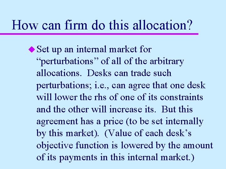
How can firm do this allocation? u Set up an internal market for “perturbations” of all of the arbitrary allocations. Desks can trade such perturbations; i. e. , can agree that one desk will lower the rhs of one of its constraints and the other will increase its. But this agreement has a price (to be set internally by this market). (Value of each desk’s objective function is lowered by the amount of its payments in this internal market. )

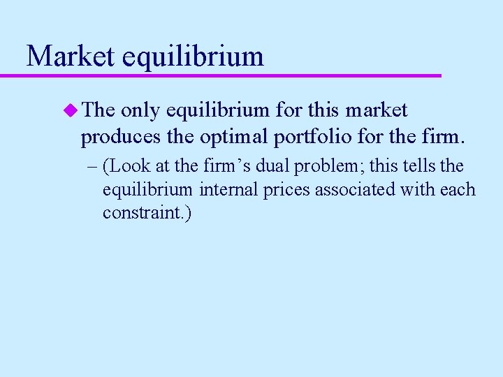
Market equilibrium u The only equilibrium for this market produces the optimal portfolio for the firm. – (Look at the firm’s dual problem; this tells the equilibrium internal prices associated with each constraint. )

What if each desk has its own Pd? u If there is some P such that EPd(X) = EP(X) for all X Î Xd then any market equilibrium solves the firm’s LP for this measure P. u If there isn’t then there is “internal arbitrage” and no market equilibrium exists.