Classification with Decision Trees I Instructor Qiang Yang

Classification with Decision Trees I Instructor: Qiang Yang Hong Kong University of Science and Technology Qyang@cs. ust. hk Thanks: Eibe Frank and Jiawei Han 1

INTRODUCTION n n Given a set of pre-classified examples, build a model or classifier to classify new cases. Supervised learning in that classes are known for the examples used to build the classifier. A classifier can be a set of rules, a decision tree, a neural network, etc. Typical Applications: credit approval, target marketing, fraud detection, medical diagnosis, treatment effectiveness analysis, …. .

Constructing a Classifier n n The goal is to maximize the accuracy on new cases that have similar class distribution. Since new cases are not available at the time of construction, the given examples are divided into the testing set and the training set. The classifier is built using the training set and is evaluated using the testing set. The goal is to be accurate on the testing set. It is essential to capture the “structure” shared by both sets. Must prune overfitting rules that work well on the training set, but poorly on the testing set. 3

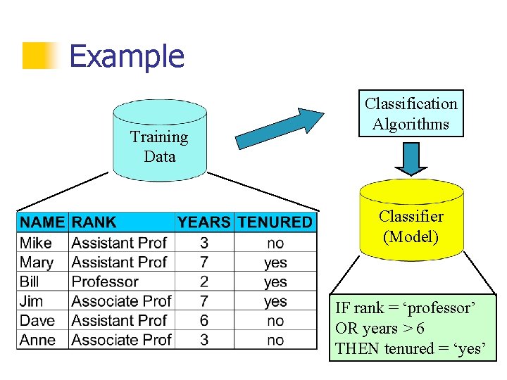
Example Training Data Classification Algorithms Classifier (Model) IF rank = ‘professor’ OR years > 6 THEN tenured = ‘yes’

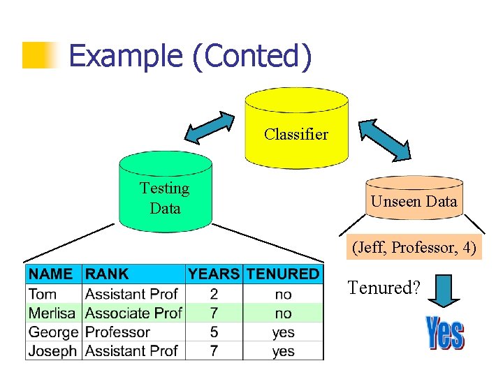
Example (Conted) Classifier Testing Data Unseen Data (Jeff, Professor, 4) Tenured?

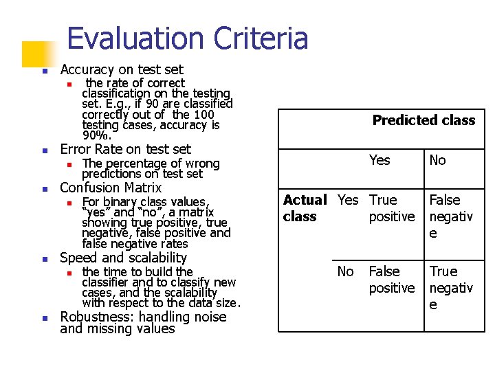
Evaluation Criteria n Accuracy on test set n n n For binary class values, “yes” and “no”, a matrix showing true positive, true negative, false positive and false negative rates Speed and scalability n Yes The percentage of wrong predictions on test set Confusion Matrix n n Predicted class Error Rate on test set n n the rate of correct classification on the testing set. E. g. , if 90 are classified correctly out of the 100 testing cases, accuracy is 90%. the time to build the classifier and to classify new cases, and the scalability with respect to the data size. Robustness: handling noise and missing values No Actual Yes True class positive False negativ e No True negativ e False positive

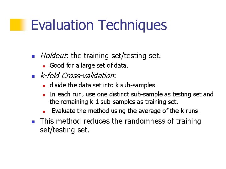
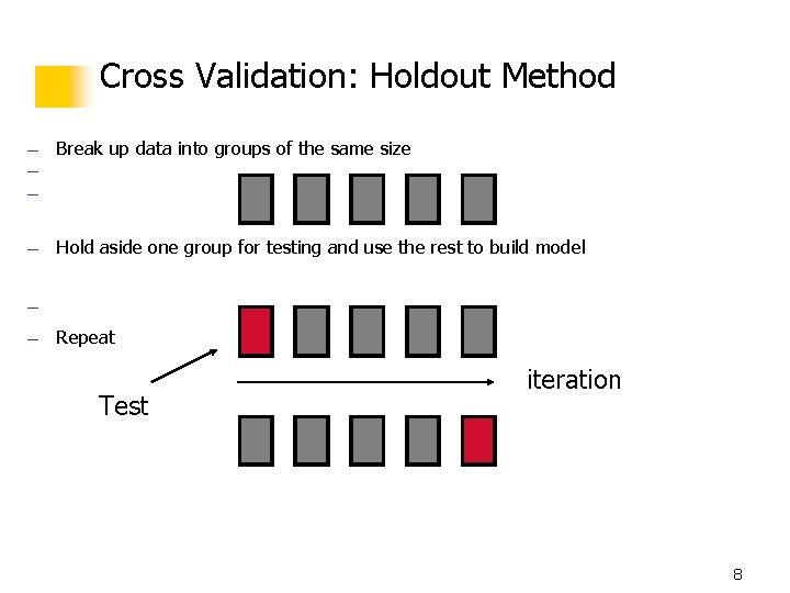
Evaluation Techniques n Holdout: the training set/testing set. n n k-fold Cross-validation: n n Good for a large set of data. divide the data set into k sub-samples. In each run, use one distinct sub-sample as testing set and the remaining k-1 sub-samples as training set. Evaluate the method using the average of the k runs. This method reduces the randomness of training set/testing set.

Cross Validation: Holdout Method — Break up data into groups of the same size — — — Hold aside one group for testing and use the rest to build model — — Repeat Test iteration 8 8

Continuous Classes n Sometimes, classes are continuous in that they come from a continuous domain, n n Regression is well suited in this case: n n n e. g. , temperature or stock price. Linear and multiple regression Non-Linear regression We shall focus on categorical classes, e. g. , colors or Yes/No binary decisions. n We will deal with continuous class values later in CART 9

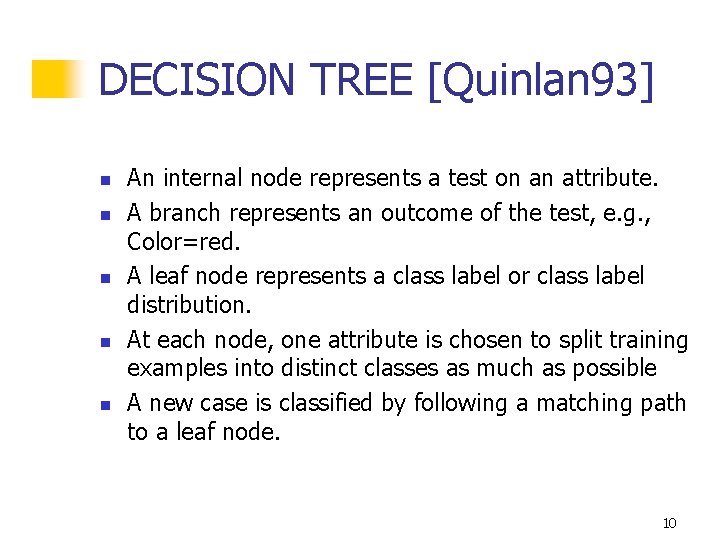
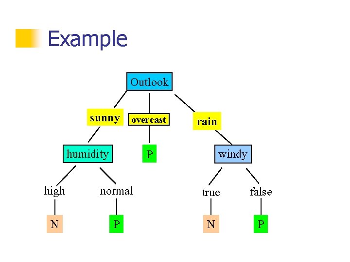
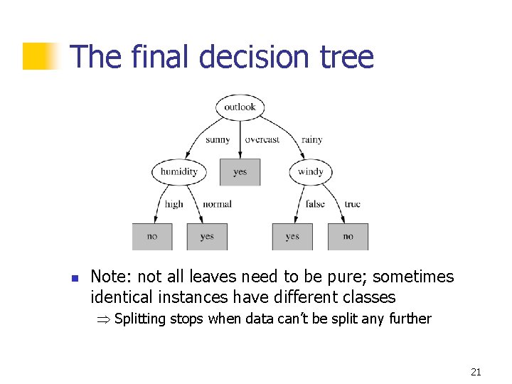
DECISION TREE [Quinlan 93] n n n An internal node represents a test on an attribute. A branch represents an outcome of the test, e. g. , Color=red. A leaf node represents a class label or class label distribution. At each node, one attribute is chosen to split training examples into distinct classes as much as possible A new case is classified by following a matching path to a leaf node. 10

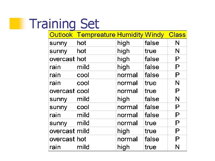
Training Set

Example Outlook sunny overcast humidity rain windy P high normal true false N P

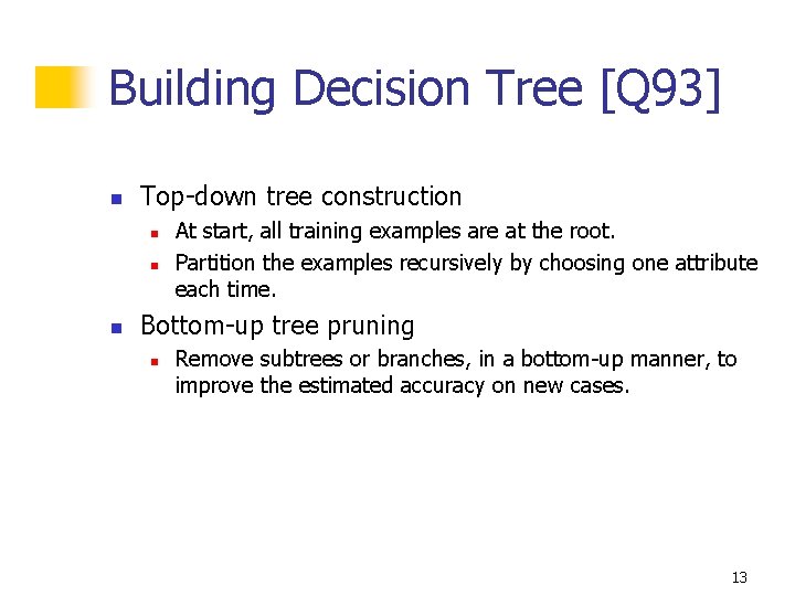
Building Decision Tree [Q 93] n Top-down tree construction n At start, all training examples are at the root. Partition the examples recursively by choosing one attribute each time. Bottom-up tree pruning n Remove subtrees or branches, in a bottom-up manner, to improve the estimated accuracy on new cases. 13

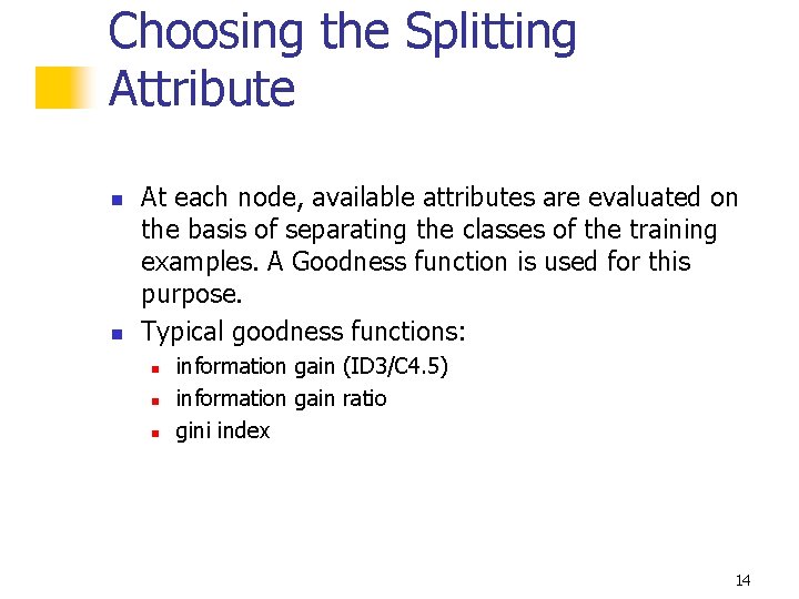
Choosing the Splitting Attribute n n At each node, available attributes are evaluated on the basis of separating the classes of the training examples. A Goodness function is used for this purpose. Typical goodness functions: n n n information gain (ID 3/C 4. 5) information gain ratio gini index 14

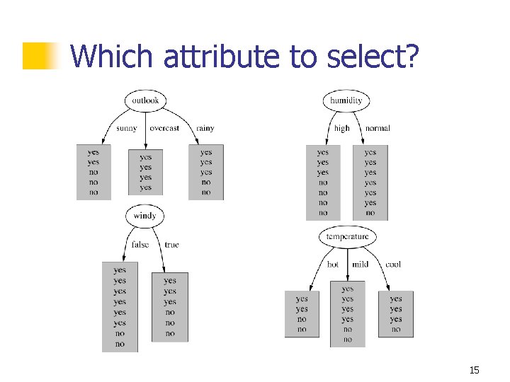
Which attribute to select? 15

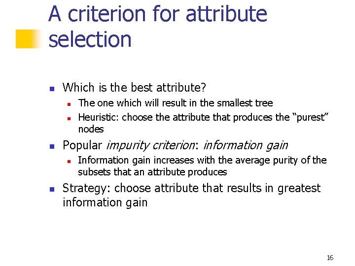
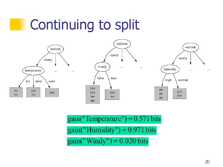
A criterion for attribute selection n Which is the best attribute? n n n Popular impurity criterion: information gain n n The one which will result in the smallest tree Heuristic: choose the attribute that produces the “purest” nodes Information gain increases with the average purity of the subsets that an attribute produces Strategy: choose attribute that results in greatest information gain 16

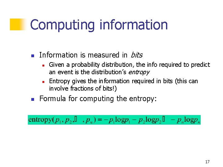
Computing information n Information is measured in bits n n n Given a probability distribution, the info required to predict an event is the distribution’s entropy Entropy gives the information required in bits (this can involve fractions of bits!) Formula for computing the entropy: 17

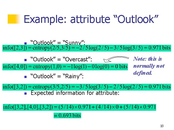
Example: attribute “Outlook” n “Outlook” = “Sunny”: n “Outlook” = “Overcast”: n “Outlook” = “Rainy”: n Expected information for attribute: Note: this is normally not defined. 18

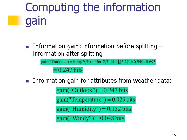
Computing the information gain n n Information gain: information before splitting – information after splitting Information gain for attributes from weather data: 19

Continuing to split 20

The final decision tree n Note: not all leaves need to be pure; sometimes identical instances have different classes Splitting stops when data can’t be split any further 21

Highly-branching attributes n n Problematic: attributes with a large number of values (extreme case: ID code) Subsets are more likely to be pure if there is a large number of values n Information gain is biased towards choosing attributes with a large number of values This may result in overfitting (selection of an attribute that is non-optimal for prediction) Another problem: fragmentation 22

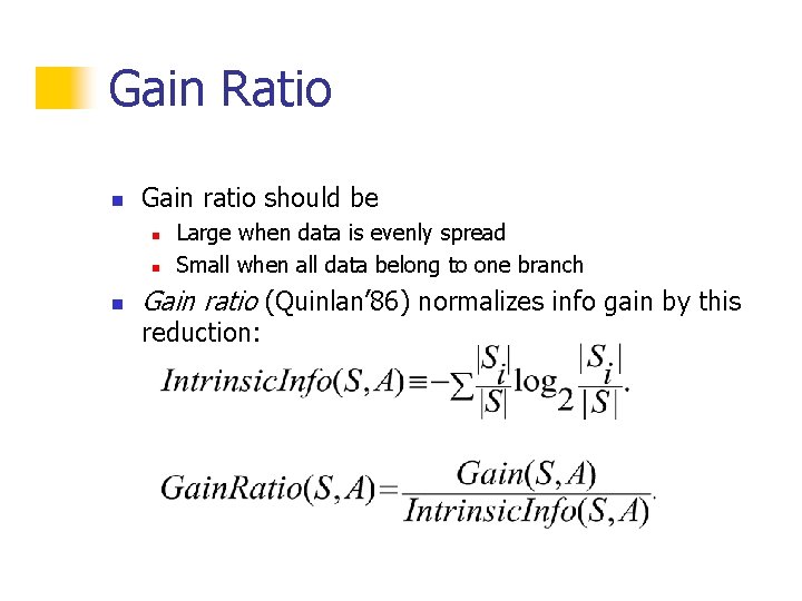
The gain ratio n n Gain ratio: a modification of the information gain that reduces its bias on high-branch attributes Gain ratio takes number and size of branches into account when choosing an attribute n n n It corrects the information gain by taking the intrinsic information of a split into account Also called split ratio Intrinsic information: entropy of distribution of instances into branches n (i. e. how much info do we need to tell which branch an instance belongs to) 23

Gain Ratio n Gain ratio should be n n n Large when data is evenly spread Small when all data belong to one branch Gain ratio (Quinlan’ 86) normalizes info gain by this reduction:

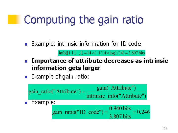
Computing the gain ratio n Example: intrinsic information for ID code n Importance of attribute decreases as intrinsic information gets larger Example of gain ratio: n Example: n 25

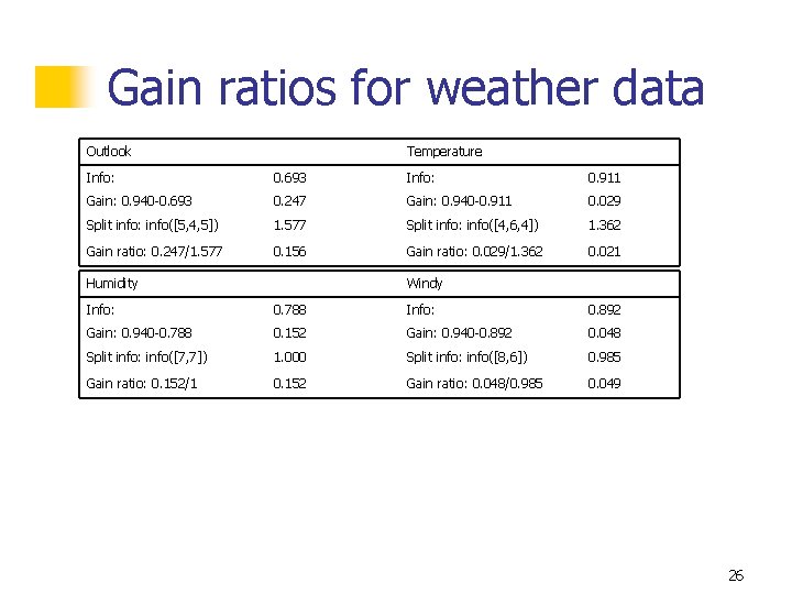
Gain ratios for weather data Outlook Temperature Info: 0. 693 Info: 0. 911 Gain: 0. 940 -0. 693 0. 247 Gain: 0. 940 -0. 911 0. 029 Split info: info([5, 4, 5]) 1. 577 Split info: info([4, 6, 4]) 1. 362 Gain ratio: 0. 247/1. 577 0. 156 Gain ratio: 0. 029/1. 362 0. 021 Humidity Windy Info: 0. 788 Info: 0. 892 Gain: 0. 940 -0. 788 0. 152 Gain: 0. 940 -0. 892 0. 048 Split info: info([7, 7]) 1. 000 Split info: info([8, 6]) 0. 985 Gain ratio: 0. 152/1 0. 152 Gain ratio: 0. 048/0. 985 0. 049 26

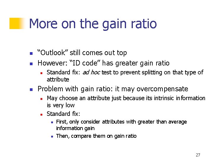
More on the gain ratio n n “Outlook” still comes out top However: “ID code” has greater gain ratio n n Standard fix: ad hoc test to prevent splitting on that type of attribute Problem with gain ratio: it may overcompensate n n May choose an attribute just because its intrinsic information is very low Standard fix: n n First, only consider attributes with greater than average information gain Then, compare them on gain ratio 27

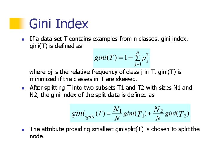
Gini Index n n n If a data set T contains examples from n classes, gini index, gini(T) is defined as where pj is the relative frequency of class j in T. gini(T) is minimized if the classes in T are skewed. After splitting T into two subsets T 1 and T 2 with sizes N 1 and N 2, the gini index of the split data is defined as The attribute providing smallest ginisplit(T) is chosen to split the node.

Discussion n Algorithm for top-down induction of decision trees (“ID 3”) was developed by Ross Quinlan n n Gain ratio just one modification of this basic algorithm Led to development of C 4. 5, which can deal with numeric attributes, missing values, and noisy data Similar approach: CART (linear regression tree, WF book, Chapter 6. 5) There are many other attribute selection criteria! (But almost no difference in accuracy of result. ) 29