Chapter Thirteen Modern Macroeconomic Models Dynamic Models A

Chapter Thirteen Modern Macroeconomic Models

Dynamic Models • A dynamic model is one in which actions that occur at one time affect what happens at other times • A static model focuses on just one point in time. • Advantages of dynamic models – Allow modeling of expectations, thus avoiding the Lucas critique – Examine how people are affected by government policy actions by including microeconomic foundations of the macroeconomy Copyright © Houghton Mifflin Company. All rights reserved. 13 | 2

Dynamic Models (cont’d) • Dynamic models are ones with microeconomic foundations, or are based on decisions of economic agents – Economic agents include households, firms, governments, and foreigners who make exchange decisions • The main disadvantage of dynamic models is that they are more complicated than static models Copyright © Houghton Mifflin Company. All rights reserved. 13 | 3

Two-period Model of Consumption & Saving The following example considers a single household and the decisions it makes in two time periods • Income is known – Period 1 income = $50, 000 – Period 2 income = $75, 000 • Can borrow or lend at fixed interest rate – Interest rate = 50 percent • There is one consumer good, which always costs $1. 00 Copyright © Houghton Mifflin Company. All rights reserved. 13 | 4

Two-period Model of Consumption & Saving (cont’d) • The household’s budget constraint – If household does not borrow or lend in period 1, spending is 50, 000 in period 1 and 75, 000 in period 2 – If household spends nothing in period 1, it saves $50, 000, invests for one year at 50%, so has $25, 000 in interest + $50, 000 principal + $75, 000 income, so can buy 150, 000 goods in period 2 Copyright © Houghton Mifflin Company. All rights reserved. 13 | 5

Two-period Model of Consumption & Saving (cont’d) Many possibilities exist for the household Period 1 • Could spend 0 -$50, 000 on goods • Could save 0 -$50, 000, earning interest • Could spend > $50, 000, borrowing at 50% interest, to be repaid in period 2 Copyright © Houghton Mifflin Company. All rights reserved. 13 | 6

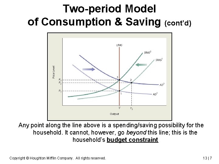
Two-period Model of Consumption & Saving (cont’d) Any point along the line above is a spending/saving possibility for the household. It cannot, however, go beyond this line; this is the household’s budget constraint Copyright © Houghton Mifflin Company. All rights reserved. 13 | 7

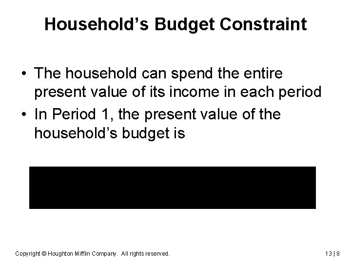
Household’s Budget Constraint • The household can spend the entire present value of its income in each period • In Period 1, the present value of the household’s budget is Copyright © Houghton Mifflin Company. All rights reserved. 13 | 8

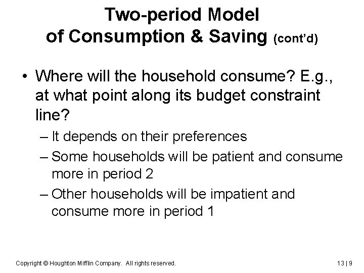
Two-period Model of Consumption & Saving (cont’d) • Where will the household consume? E. g. , at what point along its budget constraint line? – It depends on their preferences – Some households will be patient and consume more in period 2 – Other households will be impatient and consume more in period 1 Copyright © Houghton Mifflin Company. All rights reserved. 13 | 9

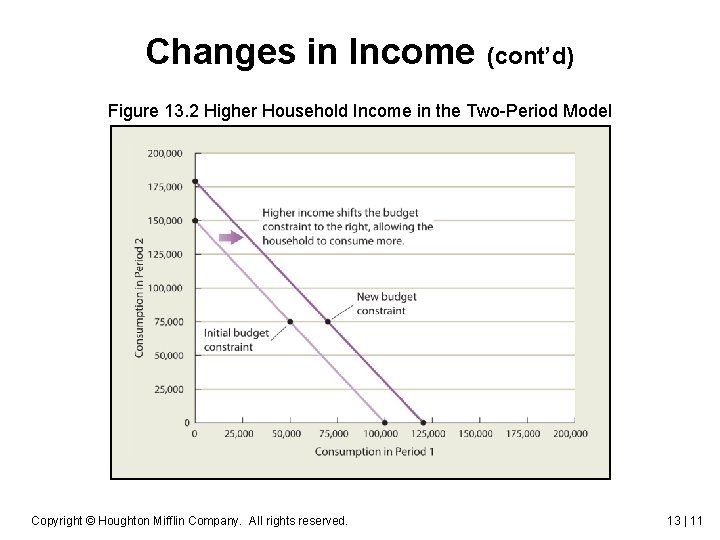
Changes in Income • Consumers with different incomes have different budget constraints • A change in income shifts the entire budget constraint • The budget constraint shifts by the exact amount as the change in income Copyright © Houghton Mifflin Company. All rights reserved. 13 | 10

Changes in Income (cont’d) Figure 13. 2 Higher Household Income in the Two-Period Model Copyright © Houghton Mifflin Company. All rights reserved. 13 | 11

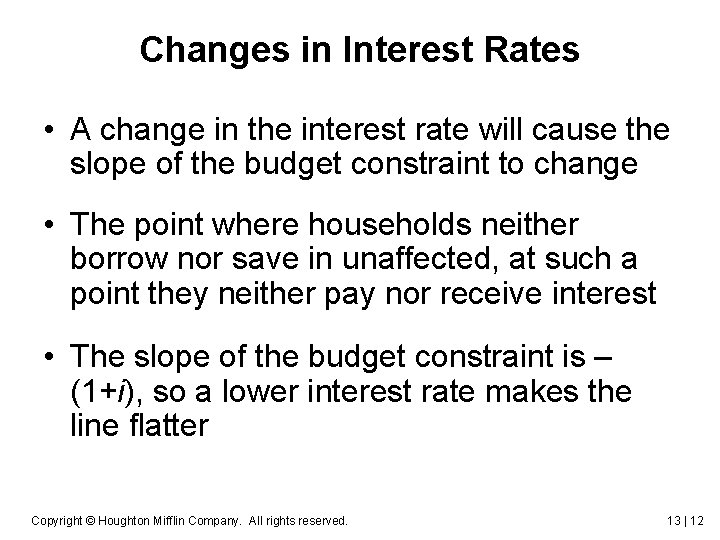
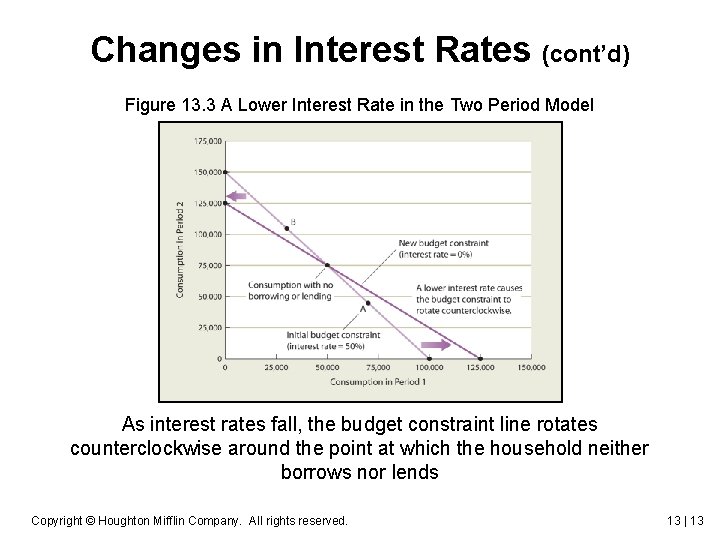
Changes in Interest Rates • A change in the interest rate will cause the slope of the budget constraint to change • The point where households neither borrow nor save in unaffected, at such a point they neither pay nor receive interest • The slope of the budget constraint is – (1+i), so a lower interest rate makes the line flatter Copyright © Houghton Mifflin Company. All rights reserved. 13 | 12

Changes in Interest Rates (cont’d) Figure 13. 3 A Lower Interest Rate in the Two Period Model As interest rates fall, the budget constraint line rotates counterclockwise around the point at which the household neither borrows nor lends Copyright © Houghton Mifflin Company. All rights reserved. 13 | 13

Changes in Interest Rates (cont’d) • Is a household better off or worse off if the interest rate is lower? – It depends on whether the household would have been a borrower or a saver at each interest rate – Someone who would have been at point A (more consumption in period 1) is better off with a lower interest rate – Someone who would have been at point B (lower consumption in period 1) is most likely worse off, but could be better off, if their preferences were such that they switched to being a borrower Copyright © Houghton Mifflin Company. All rights reserved. 13 | 14

Changes in Interest Rates (cont’d) • Consumption in each period depends on income in both periods and the interest rate – People prefer to smooth consumption spending over their lifetimes – Households anticipate future income increases, and spend more in period 1, assuming their income will be higher in period 2 – Increased income in either period likely leads to greater consumption in both periods Copyright © Houghton Mifflin Company. All rights reserved. 13 | 15

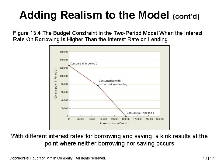
Adding Realism to the Model • The model may seem unrealistic with only two periods • It is possible to increase number of periods under analysis • In reality, households could have higher interest rates when borrowing than when lending (The budget constraint will be steeper when borrowing and flatter when saving) Copyright © Houghton Mifflin Company. All rights reserved. 13 | 16

Adding Realism to the Model (cont’d) Figure 13. 4 The Budget Constraint in the Two-Period Model When the Interest Rate On Borrowing Is Higher Than the Interest Rate on Lending With different interest rates for borrowing and saving, a kink results at the point where neither borrowing nor saving occurs Copyright © Houghton Mifflin Company. All rights reserved. 13 | 17

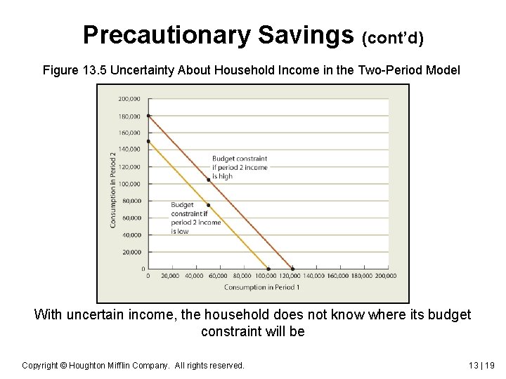
Precautionary Savings • When households are uncertain about income, they often decide to save more as a precaution • This “extra” amount of saving is known as precautionary saving • Greater uncertainty generally results in more precautionary savings • A household must therefore decide how much to spend without knowing exactly where their budget constraint will lie Copyright © Houghton Mifflin Company. All rights reserved. 13 | 18

Precautionary Savings (cont’d) Figure 13. 5 Uncertainty About Household Income in the Two-Period Model With uncertain income, the household does not know where its budget constraint will be Copyright © Houghton Mifflin Company. All rights reserved. 13 | 19

General Equilibrium • Analysis thus far has focused on single households, but should extend to the macroeconomy to be a useful model • General equilibrium is a situation in which all markets are in equilibrium and all economic agents have made decisions in their own best interest – To find general equilibrium, we need assumptions about incomes and numbers of different households and how much they decide to spend; then we must find the equilibrium interest rate and the values of other endogenous variables Copyright © Houghton Mifflin Company. All rights reserved. 13 | 20

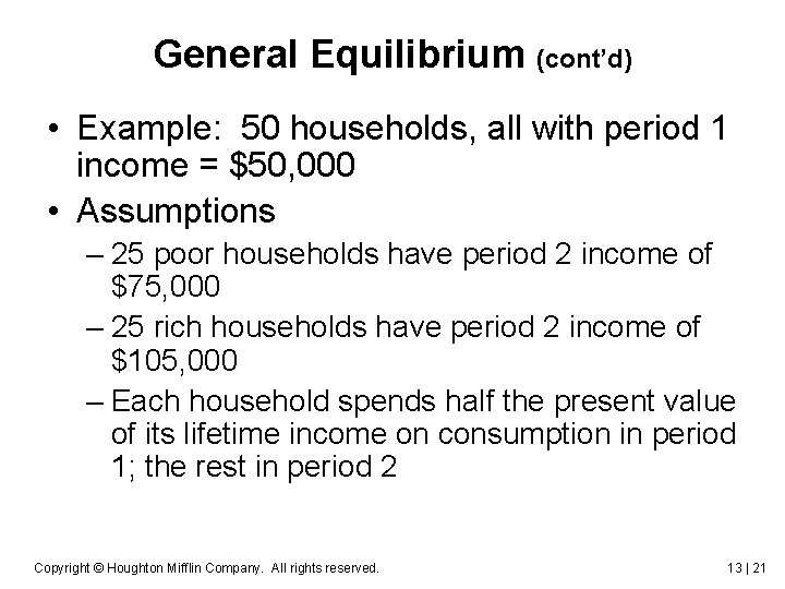
General Equilibrium (cont’d) • Example: 50 households, all with period 1 income = $50, 000 • Assumptions – 25 poor households have period 2 income of $75, 000 – 25 rich households have period 2 income of $105, 000 – Each household spends half the present value of its lifetime income on consumption in period 1; the rest in period 2 Copyright © Houghton Mifflin Company. All rights reserved. 13 | 21

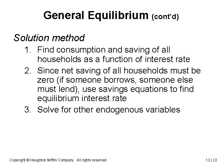
General Equilibrium (cont’d) Solution method 1. Find consumption and saving of all households as a function of interest rate 2. Since net saving of all households must be zero (if someone borrows, someone else must lend), use savings equations to find equilibrium interest rate 3. Solve for other endogenous variables Copyright © Houghton Mifflin Company. All rights reserved. 13 | 22

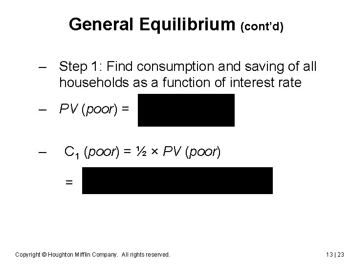
General Equilibrium (cont’d) – Step 1: Find consumption and saving of all households as a function of interest rate – PV (poor) = – C 1 (poor) = ½ × PV (poor) = Copyright © Houghton Mifflin Company. All rights reserved. 13 | 23

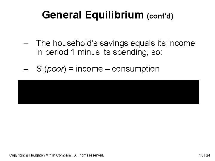
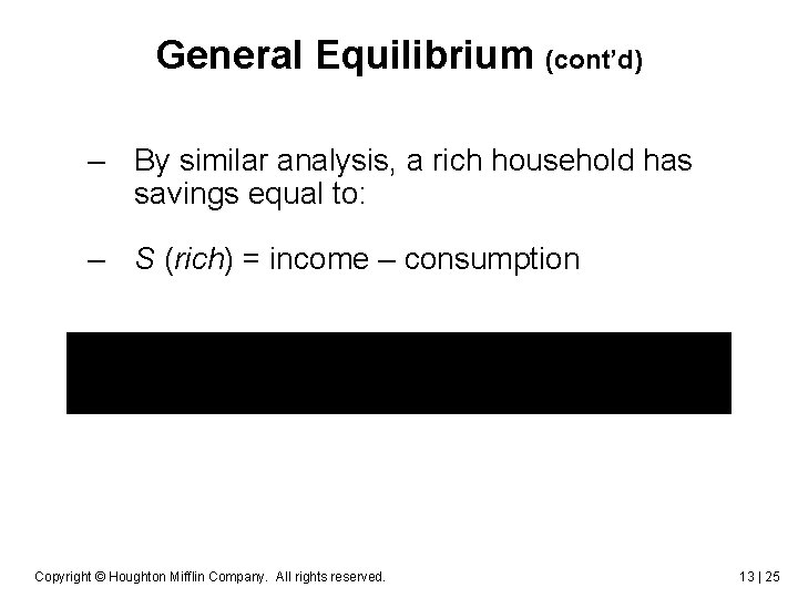
General Equilibrium (cont’d) – The household’s savings equals its income in period 1 minus its spending, so: – S (poor) = income – consumption Copyright © Houghton Mifflin Company. All rights reserved. 13 | 24

General Equilibrium (cont’d) – By similar analysis, a rich household has savings equal to: – S (rich) = income – consumption Copyright © Houghton Mifflin Company. All rights reserved. 13 | 25

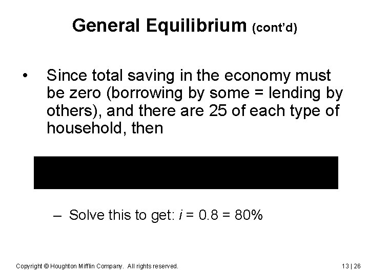
General Equilibrium (cont’d) • Since total saving in the economy must be zero (borrowing by some = lending by others), and there are 25 of each type of household, then – Solve this to get: i = 0. 8 = 80% Copyright © Houghton Mifflin Company. All rights reserved. 13 | 26

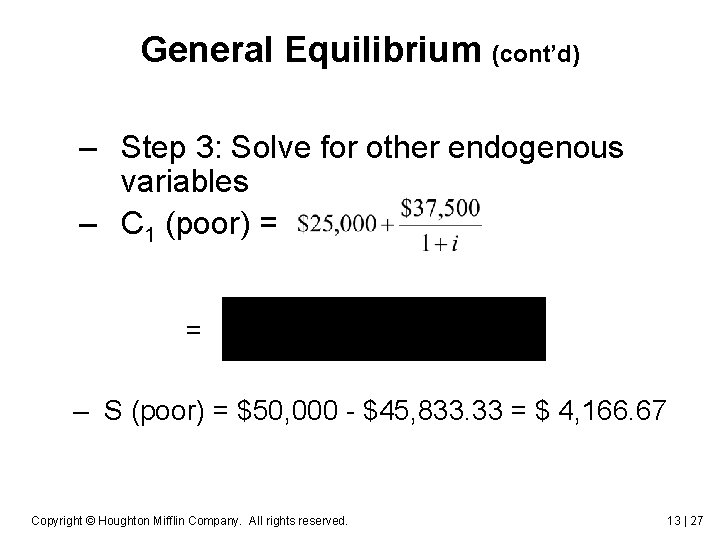
General Equilibrium (cont’d) – Step 3: Solve for other endogenous variables – C 1 (poor) = = – S (poor) = $50, 000 - $45, 833. 33 = $ 4, 166. 67 Copyright © Houghton Mifflin Company. All rights reserved. 13 | 27

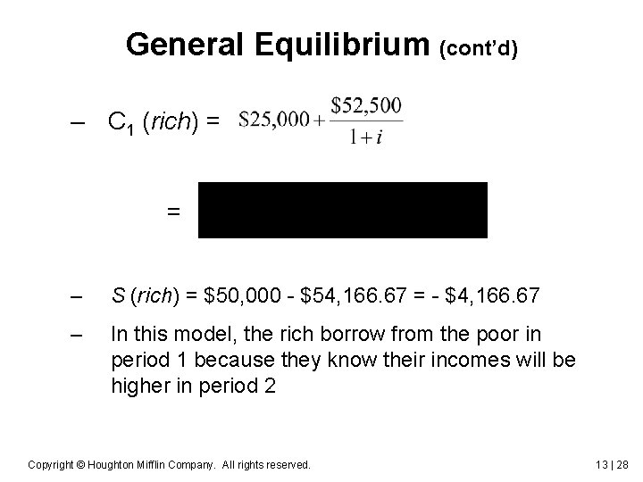
General Equilibrium (cont’d) – C 1 (rich) = = – S (rich) = $50, 000 - $54, 166. 67 = - $4, 166. 67 – In this model, the rich borrow from the poor in period 1 because they know their incomes will be higher in period 2 Copyright © Houghton Mifflin Company. All rights reserved. 13 | 28

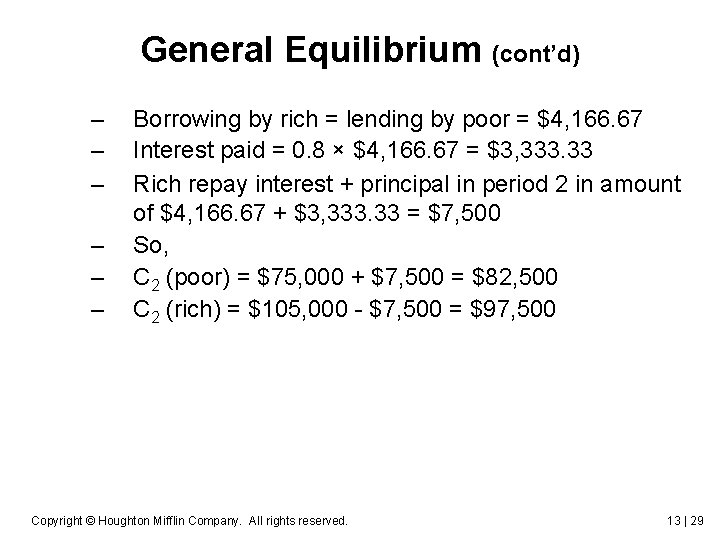
General Equilibrium (cont’d) – – – Borrowing by rich = lending by poor = $4, 166. 67 Interest paid = 0. 8 × $4, 166. 67 = $3, 333. 33 Rich repay interest + principal in period 2 in amount of $4, 166. 67 + $3, 333. 33 = $7, 500 So, C 2 (poor) = $75, 000 + $7, 500 = $82, 500 C 2 (rich) = $105, 000 - $7, 500 = $97, 500 Copyright © Houghton Mifflin Company. All rights reserved. 13 | 29

Expectations • Expectations are people’s beliefs about future economic variables – – People have rational expectations when they form expectations using all available information Expectations are best modeled as endogenous variables; decisions depend on future variables For example, households might care about future inflation and form rational expectations of inflation Since inflation depends on monetary policy, it follows that households will monitor what monetary policymakers say and do Copyright © Houghton Mifflin Company. All rights reserved. 13 | 30

The Impact of Changes in Government Policy Consider a change in fiscal policy – – Suppose the government gives everyone in the two-period model a tax rebate of $1, 000 in period 1 (household income rises by $1, 000) Do the households think the present value of their incomes has risen by $1, 000? Not if they realize that the government will increase taxes in period 2 to pay for the rebate in period 1 Realizing that the government will tax them $1, 800 in period 2 (= $1, 000 × 1. 8), people will save the entire tax rebate, as the present value of their lifetime after-tax income is unchanged Copyright © Houghton Mifflin Company. All rights reserved. 13 | 31

The Impact of Changes in Government Policy (cont’d) • The Ricardian equivalence proposition states that the result of change in the timing of taxes does not affect people’s consumption – Whether Ricardian Equivalence holds or not depends on people’s expectations and whether the present value of their income changes – Under Ricardian Equivalence, a government tax rebate has no effect; people just save the rebate, so it does not lead to increased spending – Under some conditions, such as different interest rates on borrowing and lending, or if people are unable to borrow, or if people have uncertain future incomes, Ricardian Equivalence may not hold exactly Copyright © Houghton Mifflin Company. All rights reserved. 13 | 32

DSGE Models • Dynamic, Stochastic General-Equilibrium Models …include expectations to explain how variables change over time – Dynamic implies change over time – Stochastic means including uncertainty – General equilibrium assumes that price level, wages, and interest rates adjust to bring all markets into equilibrium – First introduced as Real Business Cycle (RBC) models Copyright © Houghton Mifflin Company. All rights reserved. 13 | 33

Real Business Cycle Models • “Real” shocks to productivity are the main determinants of business cycles • Both growth and business cycles are explained by movements of a single variable- total factor productivity (TFP) • The level of TFP is the engine of growth; fluctuations in TFP generate business cycles Copyright © Houghton Mifflin Company. All rights reserved. 13 | 34

Real Business Cycle Models (cont’d) • RBC researchers used different methods than earlier macroeconomists – work with models incorporating microeconomic foundations – models are calibrated to match key business cycle facts – models are simulated on computers, not estimated with econometric analysis like other models Copyright © Houghton Mifflin Company. All rights reserved. 13 | 35

Real Business Cycle Models (cont’d) • Early RBC models were quite successful – Showed why investment spending fluctuated so much over the business cycle – Showed the close relationship between output growth and hours worked – Showed that TFP shocks accounted for about 70% of output fluctuations Copyright © Houghton Mifflin Company. All rights reserved. 13 | 36

Real Business Cycle Models (cont’d) • Some economists remained skeptical about RBC models – Government TFP data is poor, so the apparent relationship between TFP and output arises from measurement error – The data also do not reflect how intensively capital and labor are used, thus erroneously leading to correlations between output and productivity Copyright © Houghton Mifflin Company. All rights reserved. 13 | 37

Real Business Cycle Models (cont’d) • RBC theory suggests little role for government policy – TFP shocks, not government policy, are the main cause of business cycles – Government should do sensible things and stay out of the way of the private sector, keeping tax rates constant and inflation low and stable Copyright © Houghton Mifflin Company. All rights reserved. 13 | 38

Modern DSGE Models • The development of RBC models found roles for government policy, so a name change to DSGE models was in order, as models were no longer entirely “real” • Increasing power of computers allows complicated heterogeneous-agent models, with many different households, firms, etc. ; much more complicated and realistic than older homogeneous-agent models in which all agents were the same Copyright © Houghton Mifflin Company. All rights reserved. 13 | 39

Modern DSGE Models (cont’d) • Researchers using DSGE models 1. Pose the question to be answered 2. Develop a model with the core elements to be analyzed; look at the decisions made by the agents 3. Match the model to the data, and calculate the size of the shocks that occur to exogenous variables 4. Simulate the model and compare its properties to those of the data. If the model closely matches the data, answer the question in step 1. If the model does not closely match the data, modify the model and try again Copyright © Houghton Mifflin Company. All rights reserved. 13 | 40

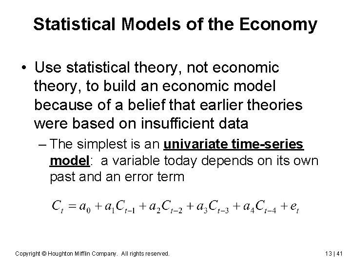
Statistical Models of the Economy • Use statistical theory, not economic theory, to build an economic model because of a belief that earlier theories were based on insufficient data – The simplest is an univariate time-series model: a variable today depends on its own past and an error term Copyright © Houghton Mifflin Company. All rights reserved. 13 | 41

Statistical Models of the Economy (cont’d) • Statistical models provide reasonably good forecasts, because the world is so complicated that dynamic models can’t capture everything • More complicated statistical models, based on many variables, do even better Copyright © Houghton Mifflin Company. All rights reserved. 13 | 42

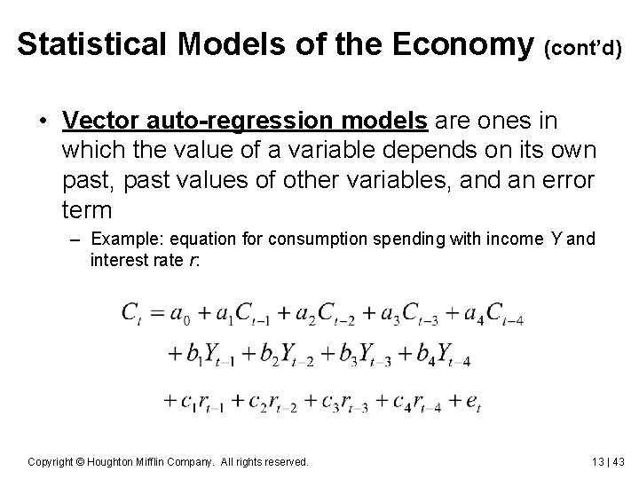
Statistical Models of the Economy (cont’d) • Vector auto-regression models are ones in which the value of a variable depends on its own past, past values of other variables, and an error term – Example: equation for consumption spending with income Y and interest rate r: Copyright © Houghton Mifflin Company. All rights reserved. 13 | 43

Vector Autoregression Models Advantages of VAR models 1. all variables are endogenous 2. can examine how a shock to one variable affects all other variables 3. can see how important one variable is in affecting movements of other variables Disadvantages of VAR models 1. hard to use them to interpret historical events 2. models lack structure, so we cannot see how some shocks affect other variables (more in next section) Copyright © Houghton Mifflin Company. All rights reserved. 13 | 44

Do Modern Macro Models Have Any Value for Policy? • Lucas critique: changes in how policy is formed may change equations of a model • So a researcher cannot take an equation that describes policy out of a large macro model or VAR model and replace it with a different equation to see how such a change would affect the economy Copyright © Houghton Mifflin Company. All rights reserved. 13 | 45

Do Modern Macro Models Have Any Value for Policy? (cont’d) • Solution for making VARs usable for policy analysis…give them some structure – Structural VAR: adds economic structure by imposing restrictions on a VAR – Short-run restrictions: how variables affect each other in the short run • Example: assume that money affects output only with a lag, which is consistent with the data – Long-run restrictions: how a change in one variable today affects another in the distant future • Example: money does not affect output in the long run, according to both theory and data Copyright © Houghton Mifflin Company. All rights reserved. 13 | 46

Do Modern Macro Models Have Any Value for Policy? • A structural VAR with long-run and shortrun restrictions provided by theory and data, provides a better interpretation of what happens to the economy when policy changes • Eventually, economists will build models usable forecasting, policy analysis, and interpreting historical events Copyright © Houghton Mifflin Company. All rights reserved. 13 | 47