Chapter 9 Aggregate Demand Economic Fluctuations Dnhaupt Dullien

Chapter 9 Aggregate Demand Economic Fluctuations © Dünhaupt, Dullien, Goodwin, Harris, Nelson, Roach, Torras

Learning Goals § After today‘s lecture, you will be able to: – Describe how unemployment and inflation behave over the business cycle. – Model consumption and investment, the components of aggregate demand – Describe the problem that “leakages” present for maintaining aggregate demand, and the classical and Keynesian approaches to leakages. – Understand how the equilibrium levels of income, consumption, investment, and savings are determined in the Keynesian model – Explain how, in the Keynesian model, the macroeconomy can equilibrate at a less- than-full-employment output level. – Describe the workings of “the multiplier, ” in words and equations. Chapter 5 2

Chapter Outline The Business Cycle 2. Macroeconomic Modeling and Aggregate Demand 1. (including the Classical Model) 3. The Keynesian Model Chapter 9 3

What makes an economy experience … GDP expansion or contraction? § high or low employment? § good or bad business conditions? § Chapter 9 4

The Business Cycle

What happens during the Business Cycle ? Business cycles = recurrent fluctuations of recession and boom § Periods of growth (several years) interrupted by times of falling output or stagnation § Recession: two consecutive quarters of a fall in GDP Chapter 9 6

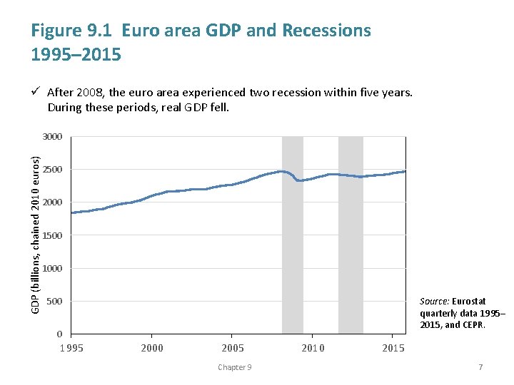
Figure 9. 1 Euro area GDP and Recessions 1995– 2015 ü After 2008, the euro area experienced two recession within five years. During these periods, real GDP fell. GDP (billions, chained 2010 euros) 3000 2500 2000 1500 1000 Source: Eurostat quarterly data 1995– 2015, and CEPR. 500 0 1995 2000 2005 Chapter 9 2010 2015 7

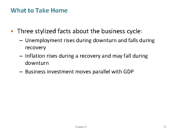
Stylized Fact #1 During an economic downturn or contraction, unemployment rises, while in a recovery or expansion, unemployment falls § If less is produced, firms need less workers § If more is produced, firms need more workers Chapter 9 8

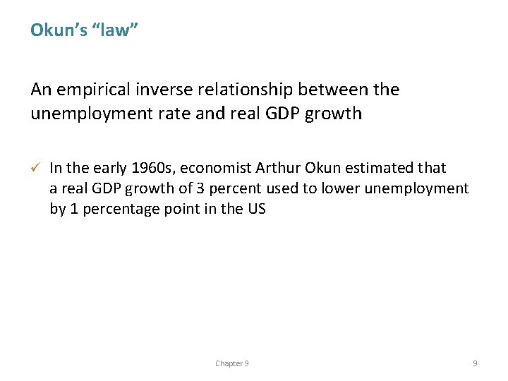
Okun’s “law” An empirical inverse relationship between the unemployment rate and real GDP growth ü In the early 1960 s, economist Arthur Okun estimated that a real GDP growth of 3 percent used to lower unemployment by 1 percentage point in the US Chapter 9 9

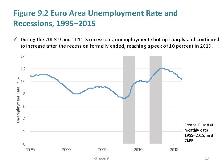
Figure 9. 2 Euro Area Unemployment Rate and Recessions, 1995– 2015 ü During the 2008 -9 and 2011 -3 recessions, unemployment shot up sharply and continued to increase after the recession formally ended, reaching a peak of 10 percent in 2010. 14 Unemployment Rate, in % 12 10 8 6 4 Source: Eurostat monthly data 1995– 2015, and CEPR. 2 0 1995 2000 2005 Chapter 9 2010 2015 10

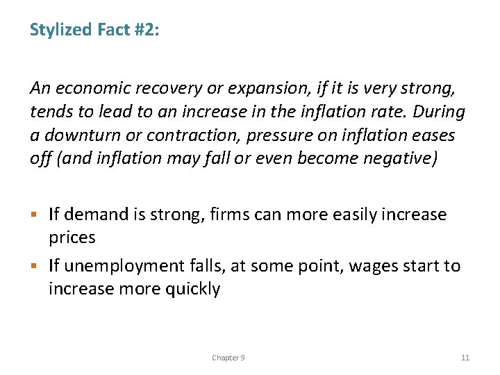
Stylized Fact #2: An economic recovery or expansion, if it is very strong, tends to lead to an increase in the inflation rate. During a downturn or contraction, pressure on inflation eases off (and inflation may fall or even become negative) If demand is strong, firms can more easily increase prices § If unemployment falls, at some point, wages start to increase more quickly § Chapter 9 11

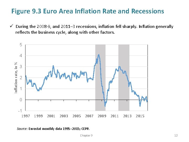
Figure 9. 3 Euro Area Inflation Rate and Recessions ü During the 2008 -9, and 2011– 3 recessions, inflation fell sharply. Inflation generally reflects the business cycle, along with other factors. 5 Inflation rate, in % 4 3 2 1 0 -1 1997 1999 2001 2003 2005 2007 2009 2011 2013 2015 Source: Eurostat monthly data 1995– 2015; CEPR. Chapter 9 12

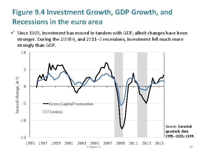
Stylized Fact #3: Over the business cycle, business investment moves in parallel with GDP, but it varies much more strongly than GDP or household consumption Chapter 9 13

Figure 9. 4 Investment Growth, GDP Growth, and Recessions in the euro area ü Since 1995, investment has moved in tandem with GDP, albeit changes have been stronger. During the 2008 -9, and 2011– 3 recessions, investment fell much more strongly than GDP. 10 Annual change, in % 5 0 -5 Gross Capital Formation Series 1 -10 -15 1997 1999 2001 2003 2005 2007 2009 2011 2013 2015 Chapter 9 Source: Eurostat quarterly data 1995– 2015; CEPR. 14

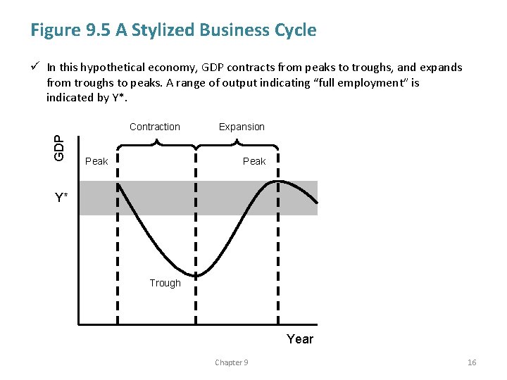
Stylized Business Cycle During a contraction, GDP falls until the economy hits the trough, or lowest point § During an expansion, GDP rises from a trough until it reaches a peak § At full-employment output, there is no problem of unemployment (though it is not zero) § goal of stabilization policy: keep economy in the gray area, avoiding threats of inflation and unemployment § Chapter 9 15

Figure 9. 5 A Stylized Business Cycle ü In this hypothetical economy, GDP contracts from peaks to troughs, and expands from troughs to peaks. A range of output indicating “full employment” is indicated by Y*. GDP Contraction Expansion Peak Y* Trough Year Chapter 9 16

The Downturn Side of the Story § The Great Depression (1929 -1939) – Stock market crash 1929 (Black Tuesday) – drop in production – increase in unemployment Chapter 9 17

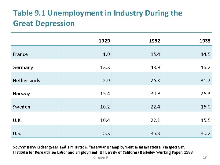
Table 9. 1 Unemployment in Industry During the Great Depression 1929 1932 1935 1. 0 15. 4 14. 5 13. 3 43. 8 16. 2 2. 9 25. 3 31. 7 Norway 15. 4 30. 8 25. 3 Sweden 10. 2 22. 4 15. 0 U. K. 10. 4 22. 1 15. 5 U. S. 5. 3 36. 3 30. 2 France Germany Netherlands Source: Barry Eichengreen and Tim Hutton, “Interwar Unemployment in International Perspective”, Institute for Research on Labor and Employment, University of California Berkeley Working Paper, 1988. Chapter 9 18

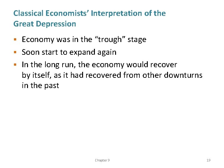
Classical Economists’ Interpretation of the Great Depression Economy was in the “trough” stage § Soon start to expand again § In the long run, the economy would recover by itself, as it had recovered from other downturns in the past § Chapter 9 19

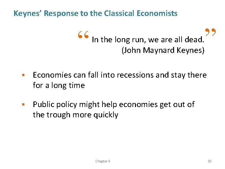
Keynes’ Response to the Classical Economists “ ” In the long run, we are all dead. (John Maynard Keynes) § Economies can fall into recessions and stay there for a long time § Public policy might help economies get out of the trough more quickly Chapter 9 20

Macroeconomic Modeling and Aggregate Demand

Simplifying Assumptions Full-employment output level does not grow § households and businesses only actors in the economy § all income in the economy goes to households § Chapter 9 22

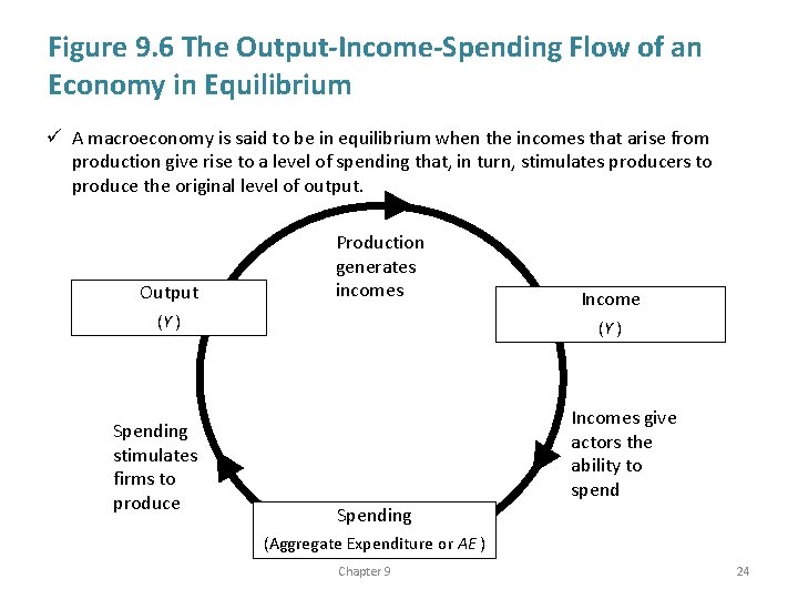
Output, Income, and Aggregate Demand “Y” represents GDP expressed as output, product, or income interchangeably § Production by firms generates labor and capital incomes to households § A macroeconomy is in an equilibrium situation when output, income, and spending are all in balance § Chapter 9 23

Figure 9. 6 The Output-Income-Spending Flow of an Economy in Equilibrium ü A macroeconomy is said to be in equilibrium when the incomes that arise from production give rise to a level of spending that, in turn, stimulates producers to produce the original level of output. Output Production generates incomes (Y ) Spending stimulates firms to produce Income (Y ) Incomes give actors the ability to spend Spending (Aggregate Expenditure or AE ) Chapter 9 24

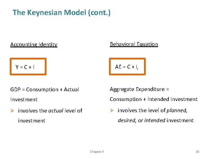
The Keynesian Model aggregate expenditure (AE) may (at least temporarily) fall out of balance with the other flows § AE depends on the spending behavior of households and firms § Household consumption C (actual spending = intended spending) § Firms investment I (actual investment ≠ intended investment II) § Chapter 9 25

The Keynesian Model (cont. ) Accounting Identity Behavioral Equation Y = C + I AE = C + II GDP = Consumption + Actual Aggregate Expenditure = Investment Consumption + Intended Investment Ø involves the actual level of Ø involves the level of planned, desired, or intended investment Chapter 9 26

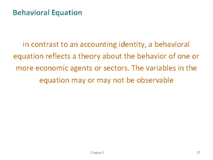
Behavioral Equation in contrast to an accounting identity, a behavioral equation reflects a theory about the behavior of one or more economic agents or sectors. The variables in the equation may or may not be observable Chapter 9 27

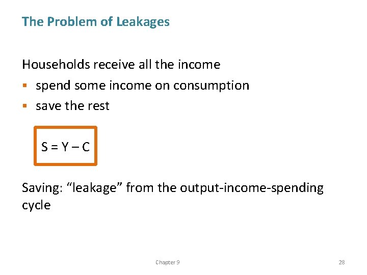
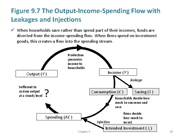
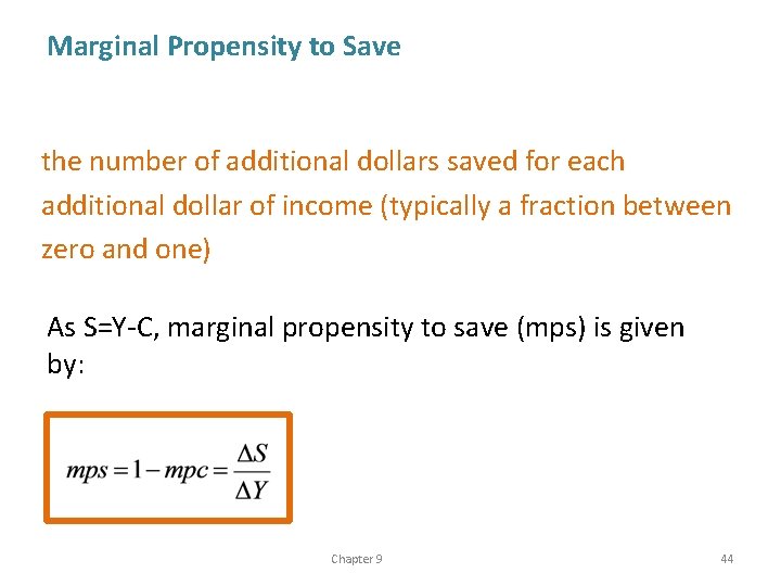
The Problem of Leakages Households receive all the income § spend some income on consumption § save the rest S = Y – C Saving: “leakage” from the output-income-spending cycle Chapter 9 28

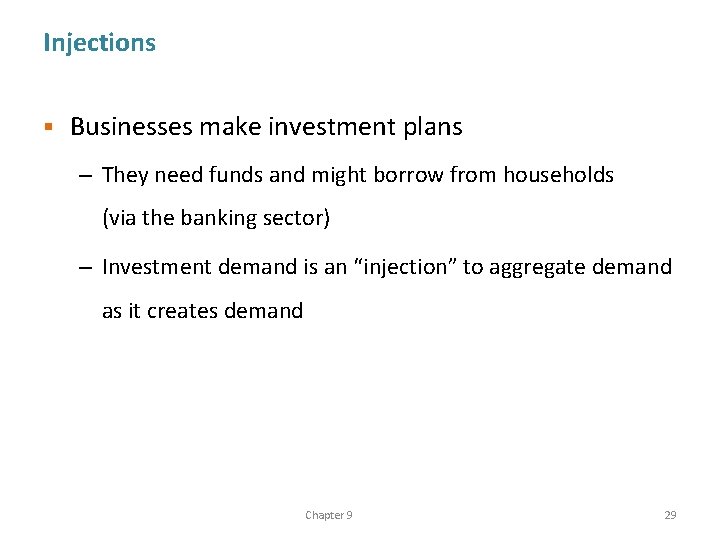
Injections § Businesses make investment plans – They need funds and might borrow from households (via the banking sector) – Investment demand is an “injection” to aggregate demand as it creates demand Chapter 9 29

Figure 9. 7 The Output-Income-Spending Flow with Leakages and Injections ü When households save rather than spend part of their incomes, funds are diverted from the income-spending flow. When firms spend on investment goods, this creates a flow into the spending stream. Production generates income to households Output (Y ) Income (Y ) leakage Sufficient to sustain output at a steady level ? Consumption (C ) Saving (S ) households decide how much to consume and save Spending (AE ) injection Chapter 9 firms decide how much to invest Intended Investment ( II ) 30

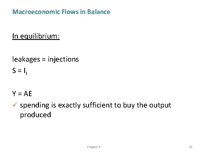
Macroeconomic Flows in Balance In equilibrium: leakages = injections S = II Y = AE ü spending is exactly sufficient to buy the output produced Chapter 9 31

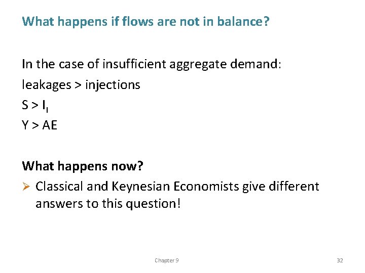
What happens if flows are not in balance? In the case of insufficient aggregate demand: leakages > injections S > II Y > AE What happens now? Ø Classical and Keynesian Economists give different answers to this question! Chapter 9 32

The Classical Solution to Leakages § Remember: In the classical world, if markets are flexible, there is only frictional unemployment – If there was unemployment, wages would fall and employment increase again Chapter 9 33

For now, we neglect the labor market and look only at another question: How does an economy keep leakages exactly equal to injections coming from investment spending? Answer: Classics argue with the “market for loanable funds” Chapter 9 34

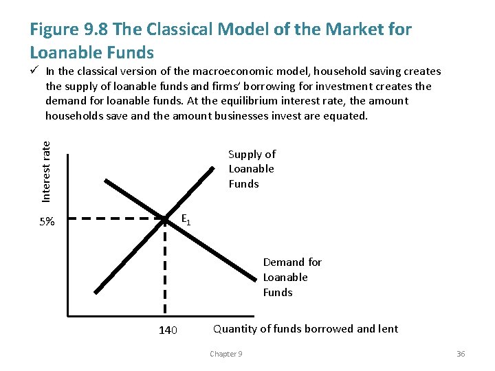
Market for Loanable Funds § Households’ saving decision based on the interest rate – High interest rate: worthwhile to save savings earn more § Firms: – the payment of interest is a cost – Low interest rates: firms borrow more for investment projects because borrowing is inexpensive – High interest rates discourage firms from borrowing Chapter 9 35

Figure 9. 8 The Classical Model of the Market for Loanable Funds Interest rate ü In the classical version of the macroeconomic model, household saving creates the supply of loanable funds and firms’ borrowing for investment creates the demand for loanable funds. At the equilibrium interest rate, the amount households save and the amount businesses invest are equated. Supply of Loanable Funds E 1 5% Demand for Loanable Funds 140 Quantity of funds borrowed and lent Chapter 9 36

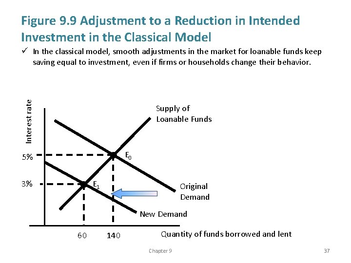
Figure 9. 9 Adjustment to a Reduction in Intended Investment in the Classical Model Interest rate ü In the classical model, smooth adjustments in the market for loanable funds keep saving equal to investment, even if firms or households change their behavior. Supply of Loanable Funds E 0 5% 3% E 1 Original Demand New Demand 60 140 Quantity of funds borrowed and lent Chapter 9 37

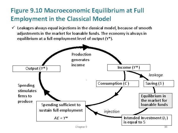
Figure 9. 10 Macroeconomic Equilibrium at Full Employment in the Classical Model ü Leakages always equal injections in the classical model, because of smooth adjustments in the market for loanable funds. The economy is always in equilibrium at a full employment level of output (Y*). Production generates income Output (Y* ) Income (Y* ) leakage Spending stimulates firms to produce Consumption (C ) Spending sufficient to sustain full employment Saving (S ) Equilibrium in the market for loanable funds injection Intended Investment (II ) is equal to S AE = Y* Chapter 9 38

Summing up the Classical Model flexible markets keep the economy at a fullemployment level of spending and output § households’ saving activity and firms’ investment spending are sensitive to changes in the interest rate (“price of loanable funds”) § an adjustment in the interest rate will quickly correct any threat of imbalances between the leakage of savings and the injection of investment. . § Ø in the Classical model, output cannot fall short of the full employment output! Chapter 9 39

The Keynesian Model

The Keynesian Model Keynes’ major contribution: develop a theory to explain why aggregate expenditure (or aggregate demand) could stay persistently low § the case of full employment (Y*) represents only a special case, one that may not often be achieved Ø He called it The General Theory § Chapter 9 41

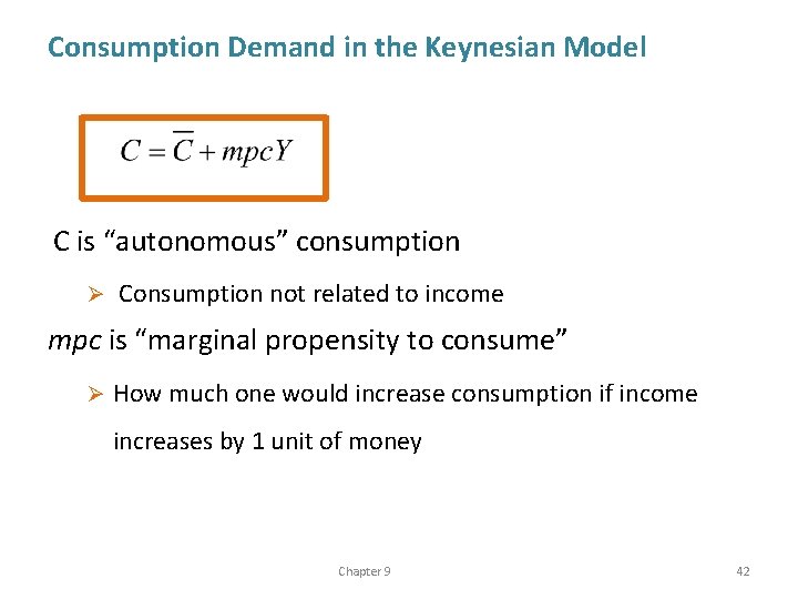
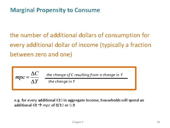
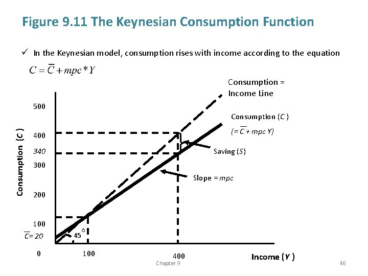
Consumption Demand in the Keynesian Model C is “autonomous” consumption Ø Consumption not related to income mpc is “marginal propensity to consume” Ø How much one would increase consumption if income increases by 1 unit of money Chapter 9 42

Marginal Propensity to Consume the number of additional dollars of consumption for every additional dollar of income (typically a fraction between zero and one) the change of C resulting from a change in Y the change in Y e. g. for every additional € 10 in aggregate income, households will spend an additional € 8 mpc of 8/10 or 0. 8 Chapter 9 43

Marginal Propensity to Save the number of additional dollars saved for each additional dollar of income (typically a fraction between zero and one) As S=Y-C, marginal propensity to save (mps) is given by: Chapter 9 44

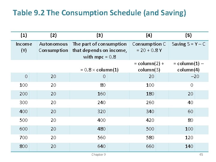
Table 9. 2 The Consumption Schedule (and Saving) (1) Income (Y) 0 (2) (3) (4) (5) Autonomous The part of consumption C Saving S = Y – C Consumption that depends on income, = 20 + 0. 8 Y with mpc = 0. 8 = column(2) + = column(1) – = 0. 8 × column(1) column(3) column(4) 20 0 20 – 20 100 20 80 100 0 20 160 180 20 300 20 240 260 40 400 20 340 60 500 20 400 420 80 600 20 480 500 100 700 20 560 580 120 800 20 640 660 140 Chapter 9 45

Figure 9. 11 The Keynesian Consumption Function ü In the Keynesian model, consumption rises with income according to the equation Consumption = Income Line 500 Consumption (C ) (= C + mpc Y) 400 340 Saving (S) 300 Slope = mpc 200 100 C= 20 0 45 100 400 Chapter 9 Income (Y ) 46

Factors That Might Impact on the Consumption Function § § § Wealth Consumer confidence Attitudes towards spending and saving Consumption-related government policies Income distribution Chapter 9 47

Classical and Keynesian Economists on Savings Classical Economics Keynesian Economics ü Saving decision depends on the interest rate ü Saving decision depends on income ü It is not sure if people save more or less if interest rates increase Chapter 9 48

Keynes on Investment Spending § Investment spending determined by: – – the cost of borrowing (the interest rate) the prices of investment goods accumulated assets and debt the willingness of people and banks to lend to them But most importantly: Ø the general level of optimism or pessimism that investors feel about the future: “animal spirits” Chapter 9 49

Keynes on Animal Spirits “ Most, probably, of our decisions to do something positive, the full consequences of which will be drawn out over many days to come, can only be taken as the result of animal spirits – a spontaneous urge to action rather than inaction, and not as the outcome of a weighted average of quantitative benefits multiplied by quantitative probabilities. (John Maynard Keynes) ” Chapter 9 50

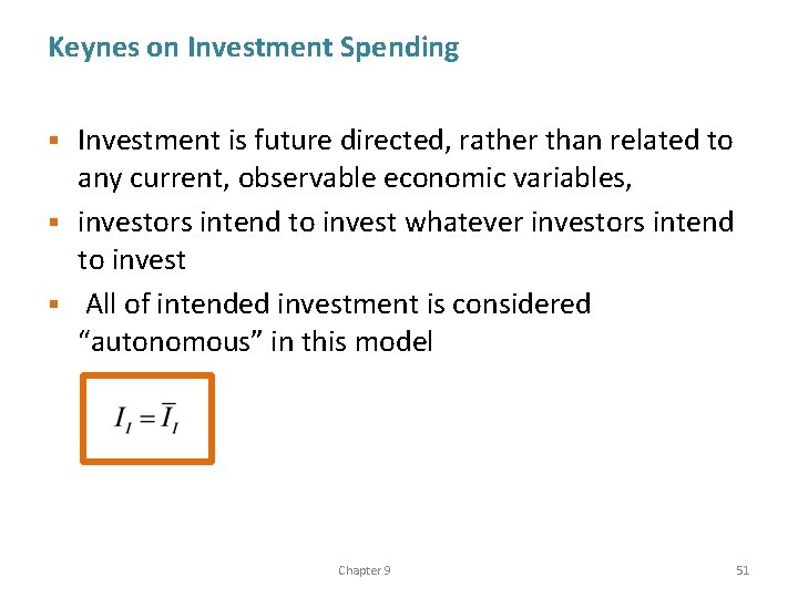
Keynes on Investment Spending Investment is future directed, rather than related to any current, observable economic variables, § investors intend to invest whatever investors intend to invest § All of intended investment is considered “autonomous” in this model § Chapter 9 51

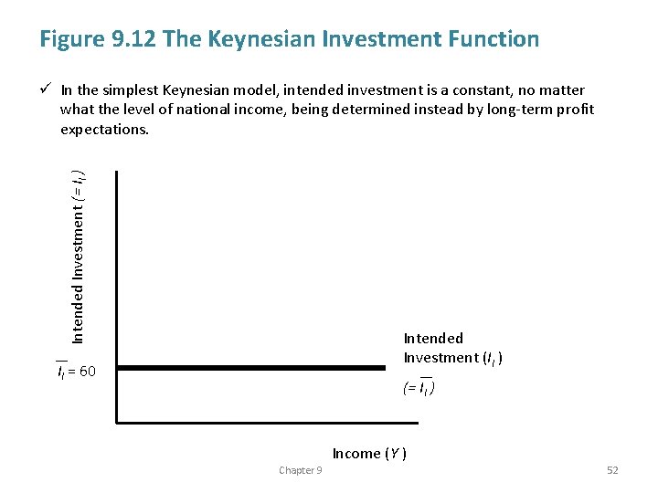
Figure 9. 12 The Keynesian Investment Function Intended Investment (= II ) ü In the simplest Keynesian model, intended investment is a constant, no matter what the level of national income, being determined instead by long-term profit expectations. Intended Investment (II ) II = 60 (= II ) Income (Y ) Chapter 9 52

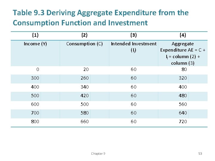
Table 9. 3 Deriving Aggregate Expenditure from the Consumption Function and Investment (1) (2) (3) Income (Y) Consumption (C) (4) Intended Investment Aggregate (II) Expenditure AE = C + II = column (2) + column (3) 60 80 0 20 300 260 60 320 400 340 60 400 500 420 60 480 600 500 60 560 700 580 60 640 800 660 60 720 Chapter 9 53

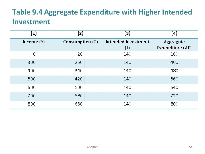
Table 9. 4 Aggregate Expenditure with Higher Intended Investment (1) (2) (3) (4) Income (Y) Consumption (C) 0 20 Intended Investment (II) 140 Aggregate Expenditure (AE) 160 300 260 140 400 340 140 480 500 420 140 560 600 500 140 640 700 580 140 720 800 660 140 800 Chapter 9 54

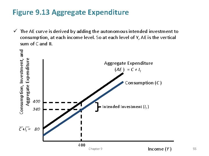
Figure 9. 13 Aggregate Expenditure Consumption, Investment, and Aggregate Expenditure ü The AE curve is derived by adding the autonomous intended investment to consumption, at each income level. So at each level of Y, AE is the vertical sum of C and II. Aggregate Expenditure (AE ) = C + II Consumption (C ) 400 Intended Investment (II ) 340 C +II = 80 400 Chapter 9 Income (Y ) 55

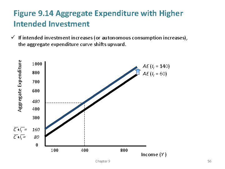
Figure 9. 14 Aggregate Expenditure with Higher Intended Investment Aggregate Expenditure ü If intended investment increases (or autonomous consumption increases), the aggregate expenditure curve shifts upward. 1000 AE (II = 140) AE (II = 60) 800 700 600 500 480 400 300 C +II = 200 160 100 80 0 100 400 800 Chapter 9 Income (Y ) 56

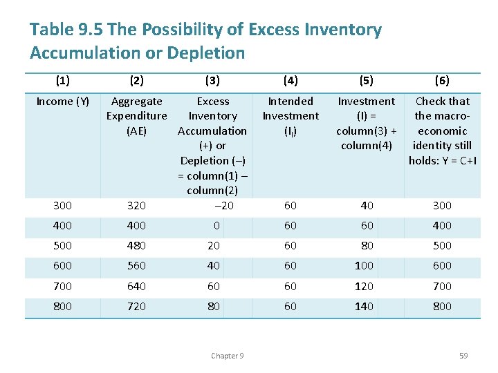
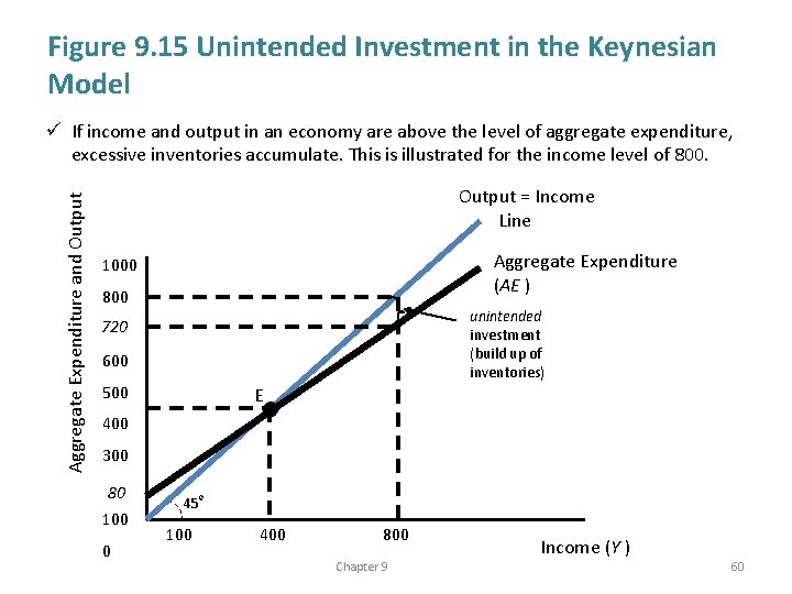
The Possibility of Unintended Investment Recall: manufactured capital stock includes structures, equipment, and inventories § There might be an unintended change in inventories: § – Unintended inventory investment: inventories build up unexpectedly – excess inventory depletion: goods “fly off the shelves” and the warehouse empties out Chapter 9 57

Actual Investment what businesses plan to invest § plus what they inadvertently end up investing if AE and Y do not match up exactly § I = intended investment (II) + excess inventory accumulation or depletion Chapter 9 58

Table 9. 5 The Possibility of Excess Inventory Accumulation or Depletion (1) Income (Y) 300 (2) (3) (4) Aggregate Excess Intended Expenditure Inventory Investment (AE) Accumulation (II) (+) or Depletion (–) = column(1) – column(2) 320 – 20 60 (5) (6) Investment (I) = column(3) + column(4) Check that the macroeconomic identity still holds: Y = C+I 40 300 400 0 60 60 400 500 480 20 60 80 500 600 560 40 60 100 600 700 640 60 60 120 700 800 720 80 60 140 800 Chapter 9 59

Figure 9. 15 Unintended Investment in the Keynesian Model Aggregate Expenditure and Output ü If income and output in an economy are above the level of aggregate expenditure, excessive inventories accumulate. This is illustrated for the income level of 800. Output = Income Line Aggregate Expenditure (AE ) 1000 800 unintended investment (build up of inventories) 720 700 600 500 E 400 300 200 80 100 0 45 100 400 800 Chapter 9 Income (Y ) 60

Movement to Equilibrium in the Keynesian Model If inventories are building up more than intended, firms cut back on production until the level of what is actually produced matches what they can sell § reductions in Y will continue until Y = AE § reduction in output leads to reduced income § which leads to reduced consumption Ø AE is a moving target changes in aggregate income, and the resulting changes in consumption and saving, cause leakages and injections to become equal again § Chapter 9 61

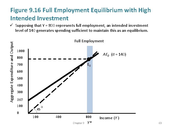
Equilibrium in Keynesian Economics Equilibrium just defines a situation in which output, spending and income are in balance § Equilibrium might be a good or a bad thing § There might be high unemployment and low unemployment equilibria § There is no mechanism which automatically brings back full employment § Chapter 9 62

Figure 9. 16 Full Employment Equilibrium with High Intended Investment Aggregate Expenditure and Output ü Supposing that Y = 800 represents full employment, an intended investment level of 140 generates spending sufficient to maintain this as an equilibrium. Full Employment 1000 AE 0 (II = 140) 800 E 0 700 600 500 400 300 200 160 100 0 45 100 400 800 Chapter 9 Y* Income (Y ) 63

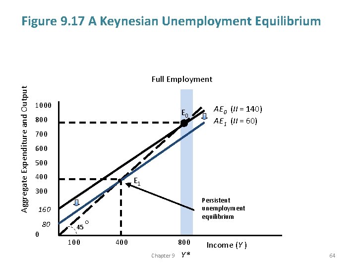
Figure 9. 17 A Keynesian Unemployment Equilibrium Aggregate Expenditure and Output Full Employment 1000 E 0 800 AE 0 (II = 140) AE 1 (II = 60) 700 600 500 400 E 1 300 200 160 100 80 0 Persistent unemployment equilibrium 45 100 400 800 Chapter 9 Y* Income (Y ) 64

A Keynesian Unemployment Equilibrium ü A fall in investor confidence causes the equilibrium level of output to fall. The initial excess of leakages over injections caused by low investment spending is corrected by a contraction in output, income, and saving. At E 1, leakages and injections are again equal. Chapter 9 65

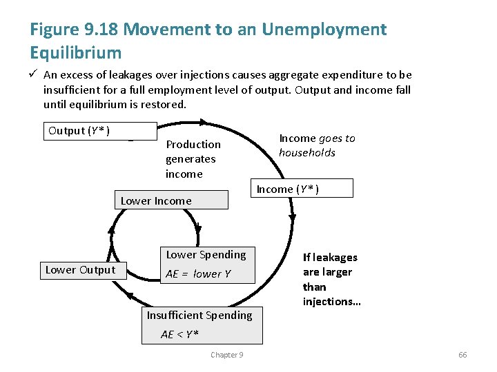
Figure 9. 18 Movement to an Unemployment Equilibrium ü An excess of leakages over injections causes aggregate expenditure to be insufficient for a full employment level of output. Output and income fall until equilibrium is restored. Output (Y* ) Production generates income Income (Y* ) Lower Income Lower Output Income goes to households Lower Spending AE = lower Y Insufficient Spending If leakages are larger than injections… AE < Y* Chapter 9 66

The Multiplier A small change in autonomous investment might bring about a large drop in output § How is this possible? § There is a multiplier effect: § – Investment creates income – Income creates consumption – Consumption creates income – Income creates consumption –… Chapter 9 67

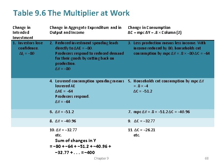
Table 9. 6 The Multiplier at Work Change in Intended Investment 1. Investors lose confidence. ΔII = − 80 Change in Aggregate Expenditure and in Output and Income Change in Consumption ΔC = mpc ΔY =. 8 × Column (2) 4. Lowered consumption spending means 5. Households cut consumption by mpc ΔY lowered AE =. 8 × − 4 ΔAE = − 64 ΔC = − 51. 2 Producers respond. ΔY = − 64 2. Reduced investment spending leads 3. Less production means less income. With directly to ΔAE = − 80. income reduced by 80, households cut Producers respond to reduced demand consumption by mpc ΔY =. 8 × − 80 ΔC = − 64 for their goods by cutting back on production. ΔY = − 80 6. ΔY = − 51. 2 7. mpc ΔY =. 8 × − 51. 2 ΔC = − 40. 96 8. ΔY = − 40. 96 9. ΔC = − 32. 77 10. ΔY = − 32. 77 etc. 11. ΔC = − 26. 21 etc. Sum of changes in Y = − 80 + − 64 + − 51. 2 + − 40. 96 + − 32. 77 +. . . = − 400 Chapter 9 68

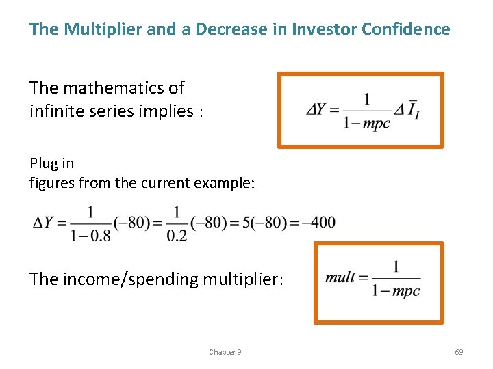
The Multiplier and a Decrease in Investor Confidence The mathematics of infinite series implies : Plug in figures from the current example: The income/spending multiplier: Chapter 9 69

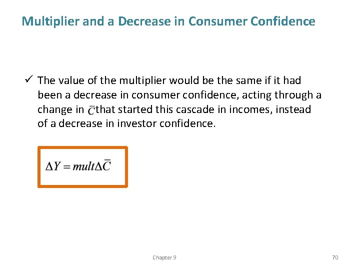
Multiplier and a Decrease in Consumer Confidence ü The value of the multiplier would be the same if it had been a decrease in consumer confidence, acting through a change in that started this cascade in incomes, instead of a decrease in investor confidence. Chapter 9 70

What to Take Home § Three stylized facts about the business cycle: – Unemployment rises during downturn and falls during recovery – Inflation rises during a recovery and may fall during downturn – Business investment moves parallel with GDP Chapter 9 71

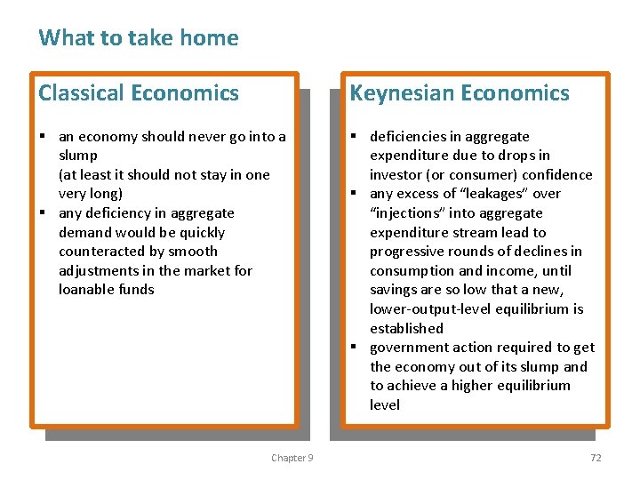
What to take home Classical Economics Keynesian Economics § an economy should never go into a slump (at least it should not stay in one very long) § any deficiency in aggregate demand would be quickly counteracted by smooth adjustments in the market for loanable funds § deficiencies in aggregate expenditure due to drops in investor (or consumer) confidence § any excess of “leakages” over “injections” into aggregate expenditure stream lead to progressive rounds of declines in consumption and income, until savings are so low that a new, lower-output-level equilibrium is established § government action required to get the economy out of its slump and to achieve a higher equilibrium level Chapter 9 72