Chapter 6 TransformandConquer Copyright 2007 Pearson AddisonWesley All

Chapter 6 Transform-and-Conquer Copyright © 2007 Pearson Addison-Wesley. All rights reserved.

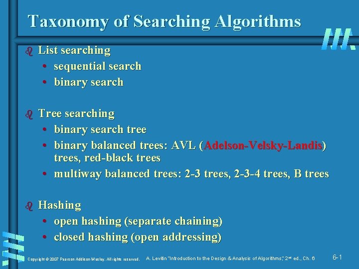
Taxonomy of Searching Algorithms b List searching • sequential search • binary search b Tree searching • binary search tree • binary balanced trees: AVL (Adelson-Velsky-Landis) trees, red-black trees • multiway balanced trees: 2 -3 trees, 2 -3 -4 trees, B trees b Hashing • open hashing (separate chaining) • closed hashing (open addressing) Copyright © 2007 Pearson Addison-Wesley. All rights reserved. A. Levitin “Introduction to the Design & Analysis of Algorithms, ” 2 nd ed. , Ch. 6 6 -1

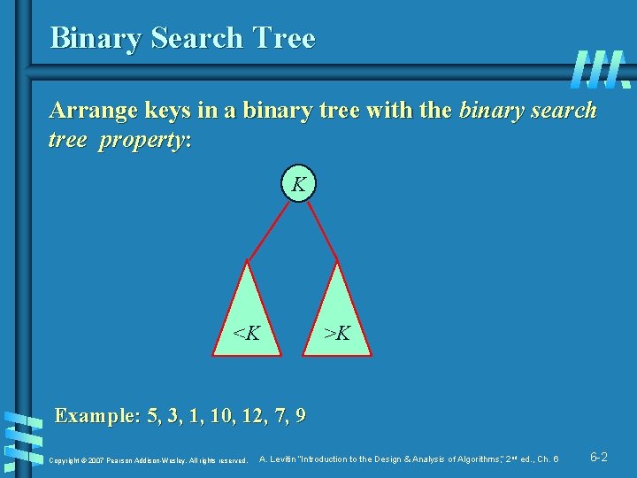
Binary Search Tree Arrange keys in a binary tree with the binary search tree property: K <K >K Example: 5, 3, 1, 10, 12, 7, 9 Copyright © 2007 Pearson Addison-Wesley. All rights reserved. A. Levitin “Introduction to the Design & Analysis of Algorithms, ” 2 nd ed. , Ch. 6 6 -2

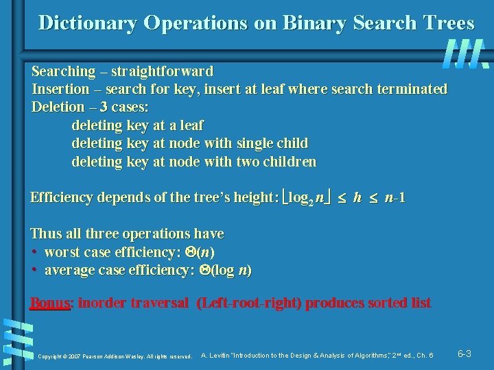
Dictionary Operations on Binary Search Trees Searching – straightforward Insertion – search for key, insert at leaf where search terminated Deletion – 3 cases: deleting key at a leaf deleting key at node with single child deleting key at node with two children Efficiency depends of the tree’s height: log 2 n h n-1 Thus all three operations have • worst case efficiency: (n) • average case efficiency: (log n) Bonus: inorder traversal (Left-root-right) produces sorted list Copyright © 2007 Pearson Addison-Wesley. All rights reserved. A. Levitin “Introduction to the Design & Analysis of Algorithms, ” 2 nd ed. , Ch. 6 6 -3

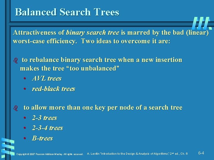
Balanced Search Trees Attractiveness of binary search tree is marred by the bad (linear) worst-case efficiency. Two ideas to overcome it are: b to rebalance binary search tree when a new insertion makes the tree “too unbalanced” • AVL trees • red-black trees b to allow more than one key per node of a search tree • 2 -3 trees • 2 -3 -4 trees • B-trees Copyright © 2007 Pearson Addison-Wesley. All rights reserved. A. Levitin “Introduction to the Design & Analysis of Algorithms, ” 2 nd ed. , Ch. 6 6 -4

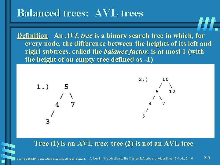
Balanced trees: AVL trees Definition An AVL tree is a binary search tree in which, for every node, the difference between the heights of its left and right subtrees, called the balance factor, is at most 1 (with the height of an empty tree defined as -1) Tree (1) is an AVL tree; tree (2) is not an AVL tree Copyright © 2007 Pearson Addison-Wesley. All rights reserved. A. Levitin “Introduction to the Design & Analysis of Algorithms, ” 2 nd ed. , Ch. 6 6 -5

Rotations If a key insertion violates the balance requirement at some node, the subtree rooted at that node is transformed via one of the four rotations. The first Assignment Question is : a) What are the types of the rotations ; give a simplified example? b) Analyze the rotation processes ? Copyright © 2007 Pearson Addison-Wesley. All rights reserved. A. Levitin “Introduction to the Design & Analysis of Algorithms, ” 2 nd ed. , Ch. 6 6 -6

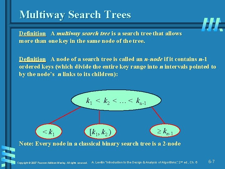
Multiway Search Trees Definition A multiway search tree is a search tree that allows more than one key in the same node of the tree. Definition A node of a search tree is called an n-node if it contains n-1 ordered keys (which divide the entire key range into n intervals pointed to by the node’s n links to its children): k 1 < k 2 < … < kn-1 < k 1 [k 1, k 2 ) kn-1 Note: Every node in a classical binary search tree is a 2 -node Copyright © 2007 Pearson Addison-Wesley. All rights reserved. A. Levitin “Introduction to the Design & Analysis of Algorithms, ” 2 nd ed. , Ch. 6 6 -7

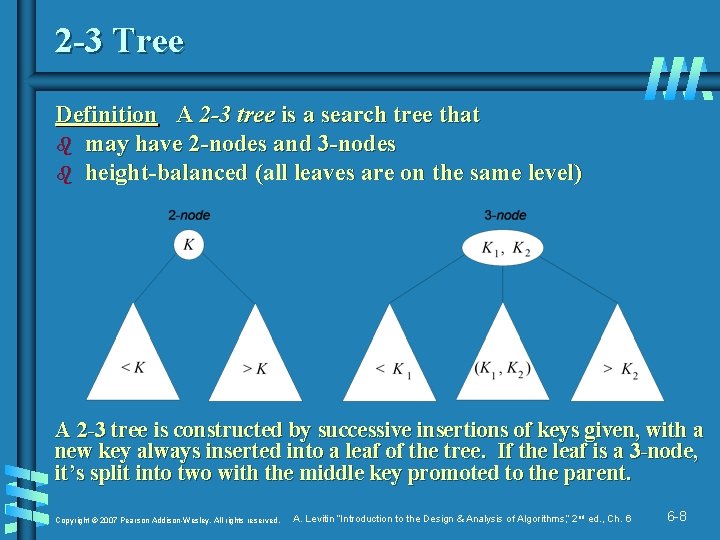
2 -3 Tree Definition A 2 -3 tree is a search tree that b may have 2 -nodes and 3 -nodes b height-balanced (all leaves are on the same level) A 2 -3 tree is constructed by successive insertions of keys given, with a new key always inserted into a leaf of the tree. If the leaf is a 3 -node, it’s split into two with the middle key promoted to the parent. Copyright © 2007 Pearson Addison-Wesley. All rights reserved. A. Levitin “Introduction to the Design & Analysis of Algorithms, ” 2 nd ed. , Ch. 6 6 -8

Construct A 2 -3 tree Video Copyright © 2007 Pearson Addison-Wesley. All rights reserved. A. Levitin “Introduction to the Design & Analysis of Algorithms, ” 2 nd ed. , Ch. 6 6 -9

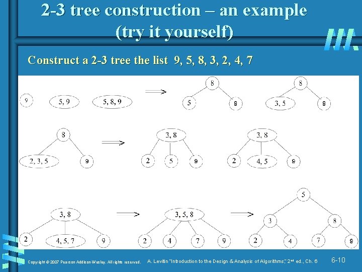
2 -3 tree construction – an example (try it yourself) Construct a 2 -3 tree the list 9, 5, 8, 3, 2, 4, 7 Copyright © 2007 Pearson Addison-Wesley. All rights reserved. A. Levitin “Introduction to the Design & Analysis of Algorithms, ” 2 nd ed. , Ch. 6 6 -10

2 nd part of assignment a) Write a program for 2 -3 tree construction ? b) Analyze the construction process? Copyright © 2007 Pearson Addison-Wesley. All rights reserved. A. Levitin “Introduction to the Design & Analysis of Algorithms, ” 2 nd ed. , Ch. 6 6 -11

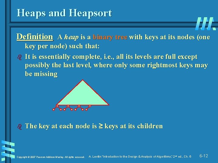
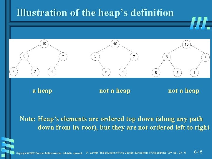
Heaps and Heapsort Definition A heap is a binary tree with keys at its nodes (one b b key per node) such that: It is essentially complete, i. e. , all its levels are full except possibly the last level, where only some rightmost keys may be missing The key at each node is ≥ keys at its children Copyright © 2007 Pearson Addison-Wesley. All rights reserved. A. Levitin “Introduction to the Design & Analysis of Algorithms, ” 2 nd ed. , Ch. 6 6 -12

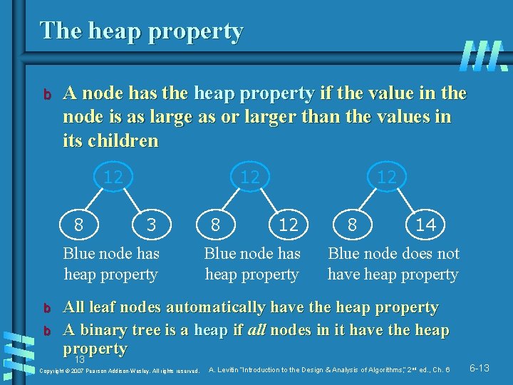
The heap property b A node has the heap property if the value in the node is as large as or larger than the values in its children 12 8 12 3 Blue node has heap property b b 8 12 12 Blue node has heap property 8 14 Blue node does not have heap property All leaf nodes automatically have the heap property A binary tree is a heap if all nodes in it have the heap property 13 Copyright © 2007 Pearson Addison-Wesley. All rights reserved. A. Levitin “Introduction to the Design & Analysis of Algorithms, ” 2 nd ed. , Ch. 6 6 -13

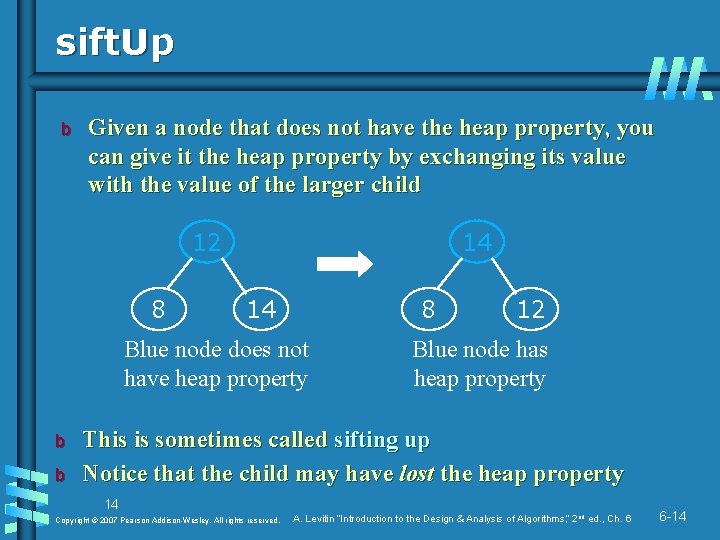
sift. Up b Given a node that does not have the heap property, you can give it the heap property by exchanging its value with the value of the larger child 12 8 14 14 8 Blue node does not have heap property b b 12 Blue node has heap property This is sometimes called sifting up Notice that the child may have lost the heap property 14 Copyright © 2007 Pearson Addison-Wesley. All rights reserved. A. Levitin “Introduction to the Design & Analysis of Algorithms, ” 2 nd ed. , Ch. 6 6 -14

Illustration of the heap’s definition a heap not a heap Note: Heap’s elements are ordered top down (along any path down from its root), but they are not ordered left to right Copyright © 2007 Pearson Addison-Wesley. All rights reserved. A. Levitin “Introduction to the Design & Analysis of Algorithms, ” 2 nd ed. , Ch. 6 6 -15

Some Important Properties of a Heap b Given n, there exists a unique binary tree with n nodes that is essentially complete, with h = log 2 n b The root contains the largest key b The subtree rooted at any node of a heap is also a heap b A heap can be represented as an array Copyright © 2007 Pearson Addison-Wesley. All rights reserved. A. Levitin “Introduction to the Design & Analysis of Algorithms, ” 2 nd ed. , Ch. 6 6 -16

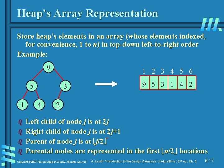
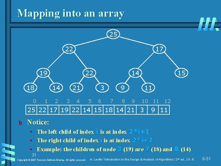
Heap’s Array Representation Store heap’s elements in an array (whose elements indexed, for convenience, 1 to n) in top-down left-to-right order Example: 9 1 2 3 4 5 6 5 1 b b 3 4 9 5 3 1 4 2 2 Left child of node j is at 2 j Right child of node j is at 2 j+1 Parent of node j is at j/2 Parental nodes are represented in the first n/2 locations Copyright © 2007 Pearson Addison-Wesley. All rights reserved. A. Levitin “Introduction to the Design & Analysis of Algorithms, ” 2 nd ed. , Ch. 6 6 -17

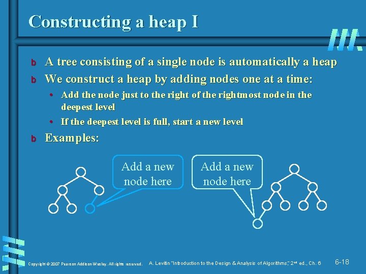
Constructing a heap I b b A tree consisting of a single node is automatically a heap We construct a heap by adding nodes one at a time: • Add the node just to the right of the rightmost node in the deepest level • If the deepest level is full, start a new level b Examples: Add a new node here Copyright © 2007 Pearson Addison-Wesley. All rights reserved. Add a new node here A. Levitin “Introduction to the Design & Analysis of Algorithms, ” 2 nd ed. , Ch. 6 6 -18

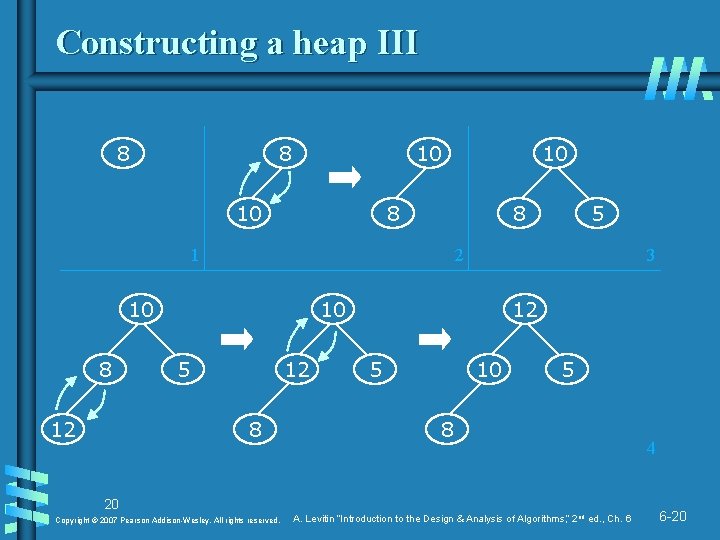
Constructing a heap II b b Each time we add a node, we may destroy the heap property of its parent node To fix this, we sift up But each time we sift up, the value of the topmost node in the sift may increase, and this may destroy the heap property of its parent node We repeat the sifting up process, moving up in the tree, until either • We reach nodes whose values don’t need to be swapped (because the parent is still larger than both children), or • We reach the root 19 Copyright © 2007 Pearson Addison-Wesley. All rights reserved. A. Levitin “Introduction to the Design & Analysis of Algorithms, ” 2 nd ed. , Ch. 6 6 -19

Constructing a heap III 8 8 10 10 8 8 1 12 5 2 10 8 10 3 10 5 12 8 12 5 10 5 8 20 Copyright © 2007 Pearson Addison-Wesley. All rights reserved. A. Levitin “Introduction to the Design & Analysis of Algorithms, ” 2 nd ed. , Ch. 6 4 6 -20

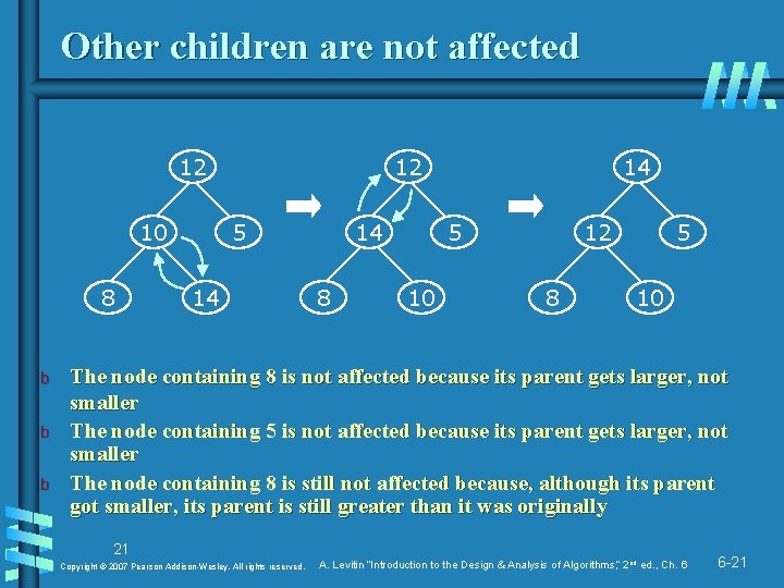
Other children are not affected 12 10 8 b b b 12 5 14 14 8 14 5 10 12 8 5 10 The node containing 8 is not affected because its parent gets larger, not smaller The node containing 5 is not affected because its parent gets larger, not smaller The node containing 8 is still not affected because, although its parent got smaller, its parent is still greater than it was originally 21 Copyright © 2007 Pearson Addison-Wesley. All rights reserved. A. Levitin “Introduction to the Design & Analysis of Algorithms, ” 2 nd ed. , Ch. 6 6 -21

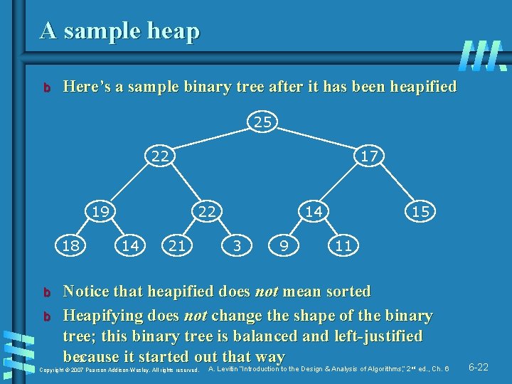
A sample heap b Here’s a sample binary tree after it has been heapified 25 22 19 18 b b 17 22 14 21 14 3 9 15 11 Notice that heapified does not mean sorted Heapifying does not change the shape of the binary tree; this binary tree is balanced and left-justified because it started out that way 22 Copyright © 2007 Pearson Addison-Wesley. All rights reserved. A. Levitin “Introduction to the Design & Analysis of Algorithms, ” 2 nd ed. , Ch. 6 6 -22

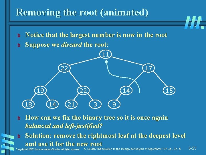
Removing the root (animated) b b Notice that the largest number is now in the root Suppose we discard the root: 11 22 19 18 b b 17 22 14 21 14 3 9 15 11 How can we fix the binary tree so it is once again balanced and left-justified? Solution: remove the rightmost leaf at the deepest level and 23 use it for the new root Copyright © 2007 Pearson Addison-Wesley. All rights reserved. A. Levitin “Introduction to the Design & Analysis of Algorithms, ” 2 nd ed. , Ch. 6 6 -23

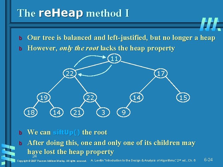
The re. Heap method I b b Our tree is balanced and left-justified, but no longer a heap However, only the root lacks the heap property 11 22 19 18 b b 17 22 14 21 14 3 15 9 We can sift. Up() the root After doing this, one and only one of its children may have lost the heap property 24 Copyright © 2007 Pearson Addison-Wesley. All rights reserved. A. Levitin “Introduction to the Design & Analysis of Algorithms, ” 2 nd ed. , Ch. 6 6 -24

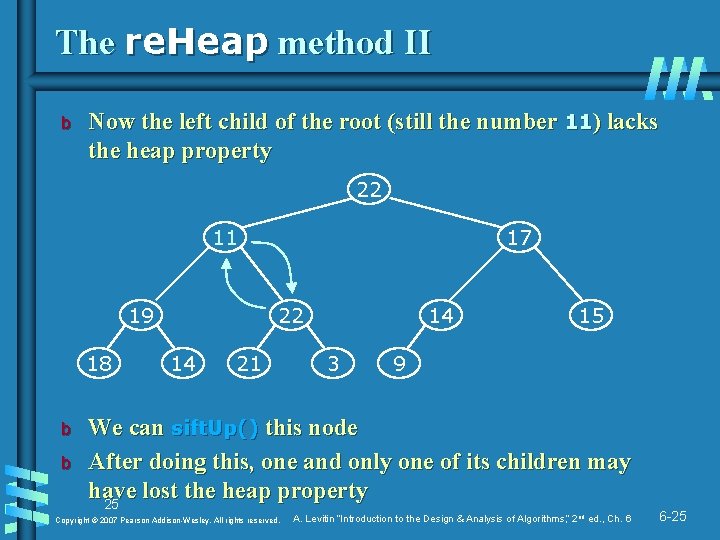
The re. Heap method II b Now the left child of the root (still the number 11) lacks the heap property 22 11 19 18 b b 17 22 14 21 14 3 15 9 We can sift. Up() this node After doing this, one and only one of its children may have lost the heap property 25 Copyright © 2007 Pearson Addison-Wesley. All rights reserved. A. Levitin “Introduction to the Design & Analysis of Algorithms, ” 2 nd ed. , Ch. 6 6 -25

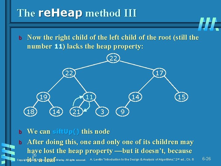
The re. Heap method III b Now the right child of the left child of the root (still the number 11) lacks the heap property: 22 22 19 18 b b 17 11 14 21 14 3 15 9 We can sift. Up() this node After doing this, one and only one of its children may have lost the heap property —but it doesn’t, because 26 A. Levitin “Introduction to the Design & Analysis of Algorithms, ” 2 ed. , Ch. 6 it’s a leaf Copyright © 2007 Pearson Addison-Wesley. All rights reserved. nd 6 -26

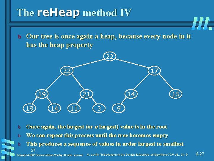
The re. Heap method IV b Our tree is once again a heap, because every node in it has the heap property 22 22 19 18 b b b 17 21 14 11 14 3 15 9 Once again, the largest (or a largest) value is in the root We can repeat this process until the tree becomes empty This produces a sequence of values in order largest to smallest 27 Copyright © 2007 Pearson Addison-Wesley. All rights reserved. A. Levitin “Introduction to the Design & Analysis of Algorithms, ” 2 nd ed. , Ch. 6 6 -27

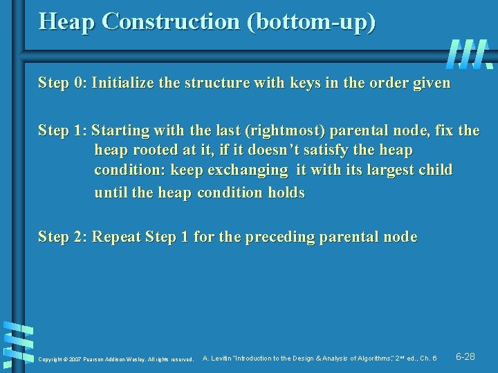
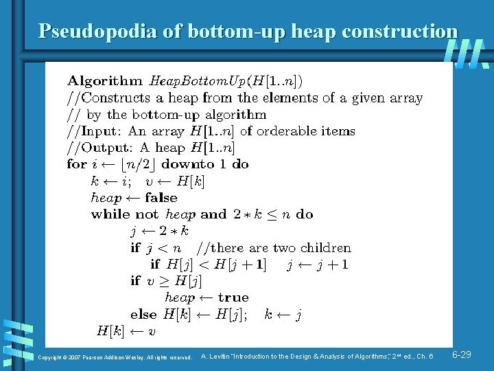
Heap Construction (bottom-up) Step 0: Initialize the structure with keys in the order given Step 1: Starting with the last (rightmost) parental node, fix the heap rooted at it, if it doesn’t satisfy the heap condition: keep exchanging it with its largest child until the heap condition holds Step 2: Repeat Step 1 for the preceding parental node Copyright © 2007 Pearson Addison-Wesley. All rights reserved. A. Levitin “Introduction to the Design & Analysis of Algorithms, ” 2 nd ed. , Ch. 6 6 -28

Pseudopodia of bottom-up heap construction Copyright © 2007 Pearson Addison-Wesley. All rights reserved. A. Levitin “Introduction to the Design & Analysis of Algorithms, ” 2 nd ed. , Ch. 6 6 -29

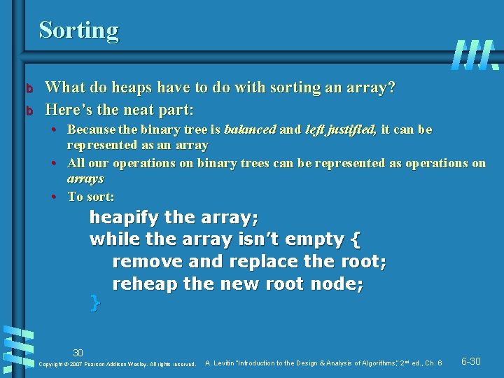
Sorting b b What do heaps have to do with sorting an array? Here’s the neat part: • Because the binary tree is balanced and left justified, it can be represented as an array • All our operations on binary trees can be represented as operations on arrays • To sort: heapify the array; while the array isn’t empty { remove and replace the root; reheap the new root node; } 30 Copyright © 2007 Pearson Addison-Wesley. All rights reserved. A. Levitin “Introduction to the Design & Analysis of Algorithms, ” 2 nd ed. , Ch. 6 6 -30

Mapping into an array 25 22 17 19 18 0 22 14 1 2 21 3 4 14 3 5 6 15 9 7 8 11 9 10 25 22 17 19 22 14 15 18 14 21 3 b 11 12 9 11 Notice: • • • 31 The left child of index i is at index 2*i+1 The right child of index i is at index 2*i+2 Example: the children of node 3 (19) are 7 (18) and 8 (14) Copyright © 2007 Pearson Addison-Wesley. All rights reserved. A. Levitin “Introduction to the Design & Analysis of Algorithms, ” 2 nd ed. , Ch. 6 6 -31

3 rd part of your assignment b How to sort the heap tree based on array representation? b Analyze the sorting? 32 Copyright © 2007 Pearson Addison-Wesley. All rights reserved. A. Levitin “Introduction to the Design & Analysis of Algorithms, ” 2 nd ed. , Ch. 6 6 -32

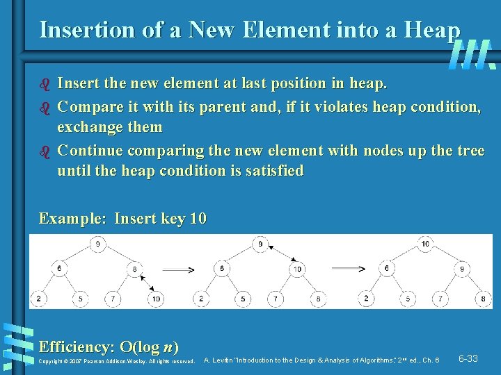
Insertion of a New Element into a Heap b b b Insert the new element at last position in heap. Compare it with its parent and, if it violates heap condition, exchange them Continue comparing the new element with nodes up the tree until the heap condition is satisfied Example: Insert key 10 Efficiency: O(log n) Copyright © 2007 Pearson Addison-Wesley. All rights reserved. A. Levitin “Introduction to the Design & Analysis of Algorithms, ” 2 nd ed. , Ch. 6 6 -33

Priority Queue A priority queue is the ADT of a set of elements with numerical priorities with the following operations: • find element with highest priority • delete element with highest priority • insert element with assigned priority (see below) b Heap is a very efficient way for implementing priority queues b Two ways to handle priority queue in which highest priority = smallest number Copyright © 2007 Pearson Addison-Wesley. All rights reserved. A. Levitin “Introduction to the Design & Analysis of Algorithms, ” 2 nd ed. , Ch. 6 6 -34

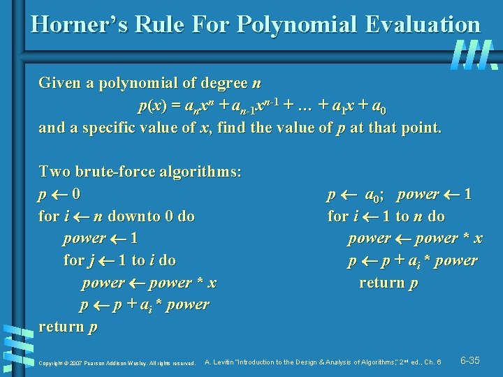
Horner’s Rule For Polynomial Evaluation Given a polynomial of degree n p(x) = anxn + an-1 xn-1 + … + a 1 x + a 0 and a specific value of x, find the value of p at that point. Two brute-force algorithms: p 0 for i n downto 0 do power 1 for j 1 to i do power * x p p + ai * power return p Copyright © 2007 Pearson Addison-Wesley. All rights reserved. p a 0; power 1 for i 1 to n do power * x p p + ai * power return p A. Levitin “Introduction to the Design & Analysis of Algorithms, ” 2 nd ed. , Ch. 6 6 -35

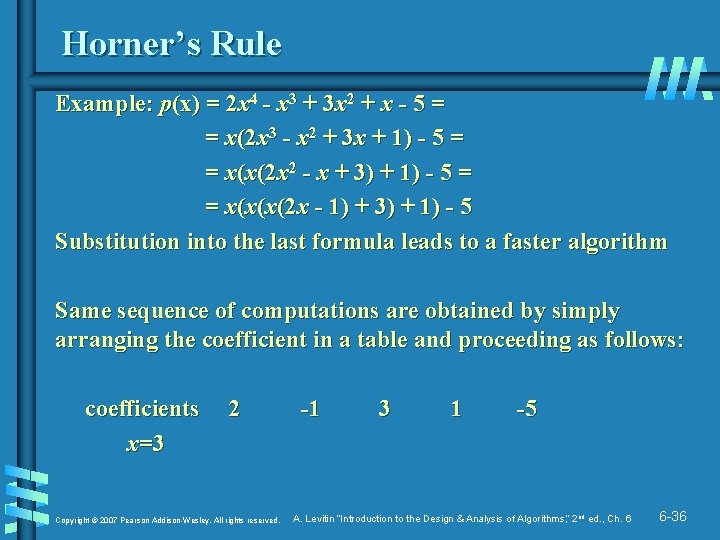
Horner’s Rule Example: p(x) = 2 x 4 - x 3 + 3 x 2 + x - 5 = = x(2 x 3 - x 2 + 3 x + 1) - 5 = = x(x(2 x 2 - x + 3) + 1) - 5 = = x(x(x(2 x - 1) + 3) + 1) - 5 Substitution into the last formula leads to a faster algorithm Same sequence of computations are obtained by simply arranging the coefficient in a table and proceeding as follows: coefficients x=3 2 Copyright © 2007 Pearson Addison-Wesley. All rights reserved. -1 3 1 -5 A. Levitin “Introduction to the Design & Analysis of Algorithms, ” 2 nd ed. , Ch. 6 6 -36

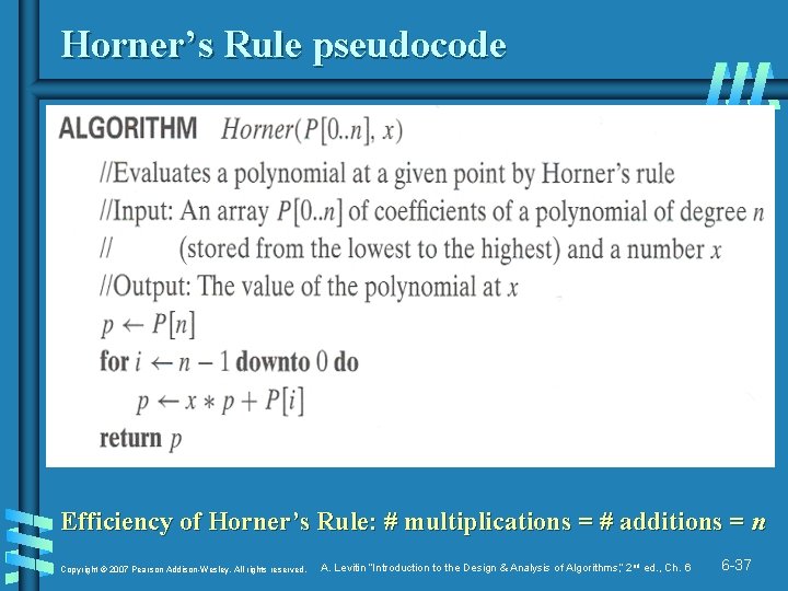
Horner’s Rule pseudocode Efficiency of Horner’s Rule: # multiplications = # additions = n Copyright © 2007 Pearson Addison-Wesley. All rights reserved. A. Levitin “Introduction to the Design & Analysis of Algorithms, ” 2 nd ed. , Ch. 6 6 -37

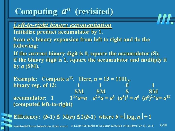
Computing an (revisited) Left-to-right binary exponentiation Initialize product accumulator by 1. Scan n’s binary expansion from left to right and do the following: If the current binary digit is 0, square the accumulator (S); if the binary digit is 1, square the accumulator and multiply it by a (SM). Example: Compute a 13. Here, n = 13 = 11012. binary rep. of 13: 1 1 0 1 SM SM S SM accumulator: 1 12*a=a a 2*a = a 3 (a 3)2 = a 6 (a 6)2*a= a 13 (computed left-to-right) Efficiency: (b-1) ≤ M(n) ≤ 2(b-1) where b = log 2 n + 1 Copyright © 2007 Pearson Addison-Wesley. All rights reserved. A. Levitin “Introduction to the Design & Analysis of Algorithms, ” 2 nd ed. , Ch. 6 6 -38

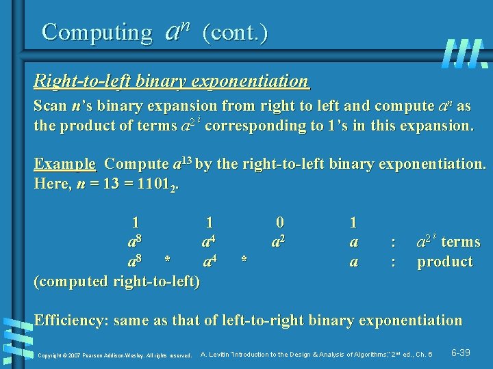
Computing an (cont. ) Right-to-left binary exponentiation Scan n’s binary expansion from right to left and compute an as the product of terms a 2 i corresponding to 1’s in this expansion. Example Compute a 13 by the right-to-left binary exponentiation. Here, n = 13 = 11012. 1 1 a 8 a 4 a 8 * a 4 (computed right-to-left) 0 a 2 * 1 a a : : a 2 i terms product Efficiency: same as that of left-to-right binary exponentiation Copyright © 2007 Pearson Addison-Wesley. All rights reserved. A. Levitin “Introduction to the Design & Analysis of Algorithms, ” 2 nd ed. , Ch. 6 6 -39

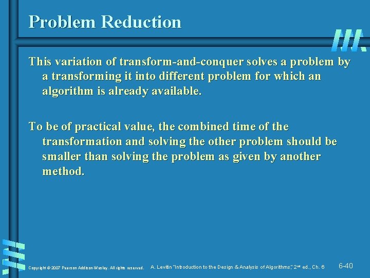
Problem Reduction This variation of transform-and-conquer solves a problem by a transforming it into different problem for which an algorithm is already available. To be of practical value, the combined time of the transformation and solving the other problem should be smaller than solving the problem as given by another method. Copyright © 2007 Pearson Addison-Wesley. All rights reserved. A. Levitin “Introduction to the Design & Analysis of Algorithms, ” 2 nd ed. , Ch. 6 6 -40

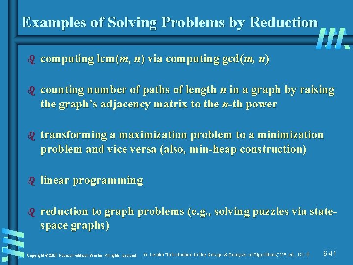
Examples of Solving Problems by Reduction b computing lcm(m, n) via computing gcd(m, n) b counting number of paths of length n in a graph by raising the graph’s adjacency matrix to the n-th power b transforming a maximization problem to a minimization problem and vice versa (also, min-heap construction) b linear programming b reduction to graph problems (e. g. , solving puzzles via statespace graphs) Copyright © 2007 Pearson Addison-Wesley. All rights reserved. A. Levitin “Introduction to the Design & Analysis of Algorithms, ” 2 nd ed. , Ch. 6 6 -41