Chapter 10 Review Day Test next class Section

Chapter 10 Review Day Test next class!!!

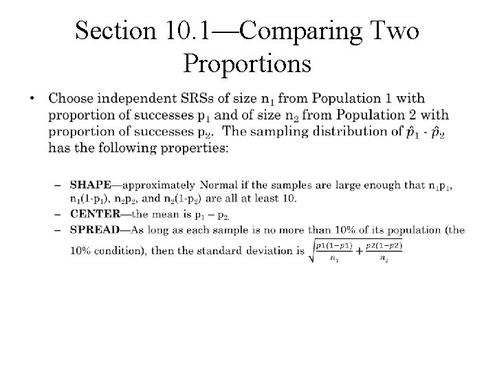
Section 10. 1—Comparing Two Proportions •

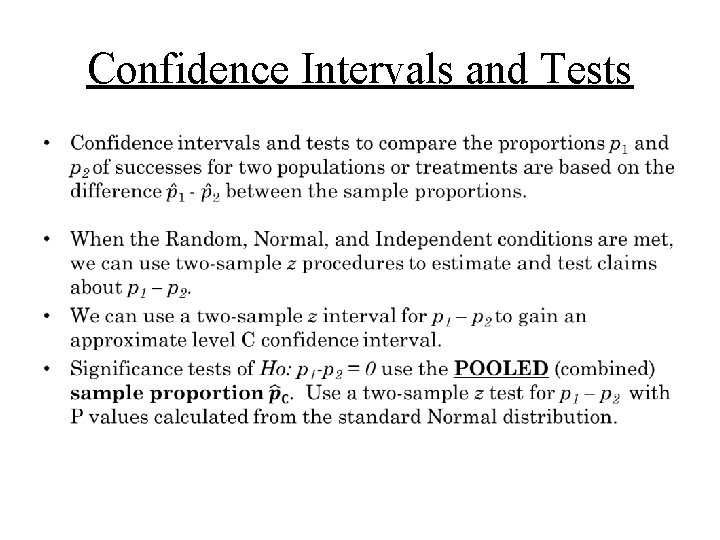
Confidence Intervals and Tests •

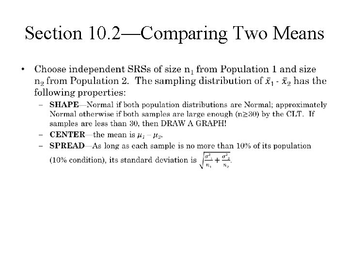
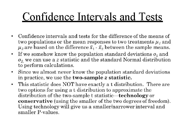
Section 10. 2—Comparing Two Means •

Confidence Intervals and Tests •

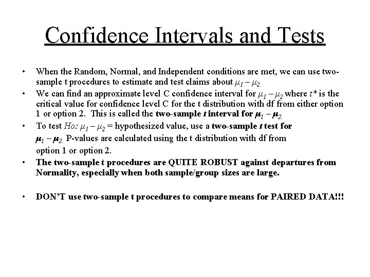
Confidence Intervals and Tests • • • When the Random, Normal, and Independent conditions are met, we can use twosample t procedures to estimate and test claims about μ 1 – μ 2. We can find an approximate level C confidence interval for μ 1 – μ 2 where t* is the critical value for confidence level C for the t distribution with df from either option 1 or option 2. This is called the two-sample t interval for μ 1 – μ 2. To test Ho: μ 1 – μ 2 = hypothesized value, use a two-sample t test for μ 1 – μ 2. P-values are calculated using the t distribution with df from option 1 or option 2. The two-sample t procedures are QUITE ROBUST against departures from Normality, especially when both sample/group sizes are large. DON’T use two-sample t procedures to compare means for PAIRED DATA!!!

For each of the following, determine: 1)Would you use a one-sample t, two -sample t, or paired t method? 2)Would you perform a hypothesis test or find a confidence interval?

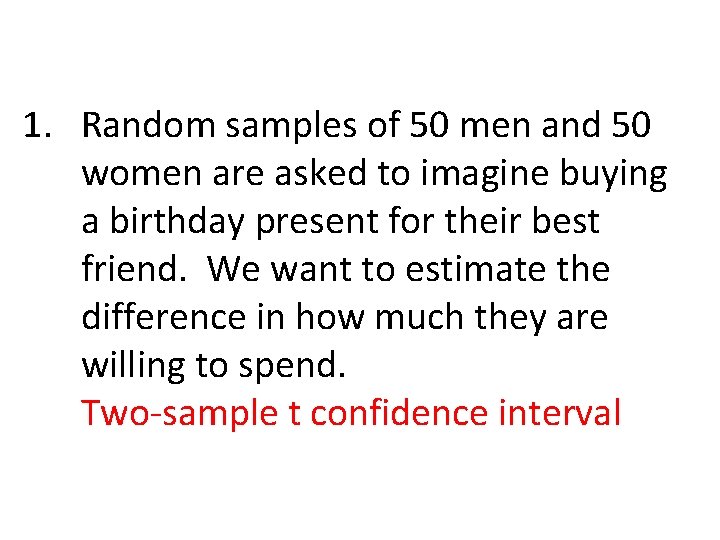
1. Random samples of 50 men and 50 women are asked to imagine buying a birthday present for their best friend. We want to estimate the difference in how much they are willing to spend. Two-sample t confidence interval

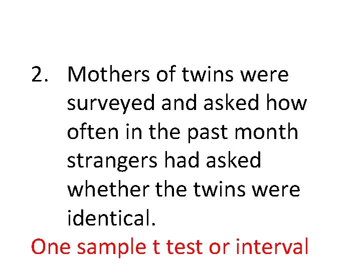
2. Mothers of twins were surveyed and asked how often in the past month strangers had asked whether the twins were identical. One sample t test or interval

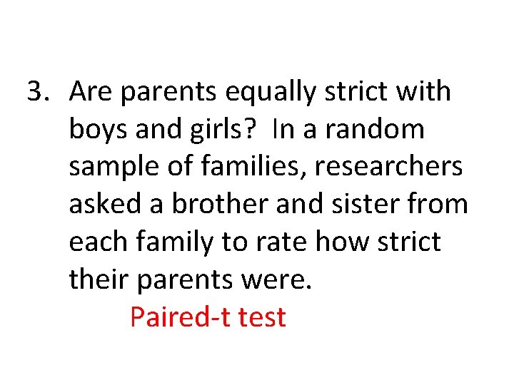
3. Are parents equally strict with boys and girls? In a random sample of families, researchers asked a brother and sister from each family to rate how strict their parents were. Paired-t test

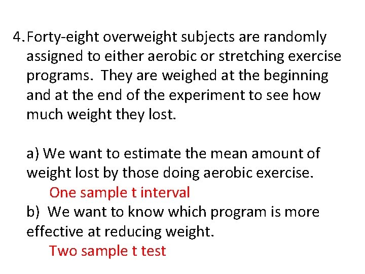
4. Forty-eight overweight subjects are randomly assigned to either aerobic or stretching exercise programs. They are weighed at the beginning and at the end of the experiment to see how much weight they lost. a) We want to estimate the mean amount of weight lost by those doing aerobic exercise. One sample t interval b) We want to know which program is more effective at reducing weight. Two sample t test

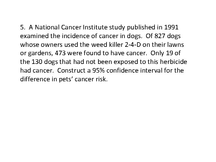
5. A National Cancer Institute study published in 1991 examined the incidence of cancer in dogs. Of 827 dogs whose owners used the weed killer 2 -4 -D on their lawns or gardens, 473 were found to have cancer. Only 19 of the 130 dogs that had not been exposed to this herbicide had cancer. Construct a 95% confidence interval for the difference in pets’ cancer risk.

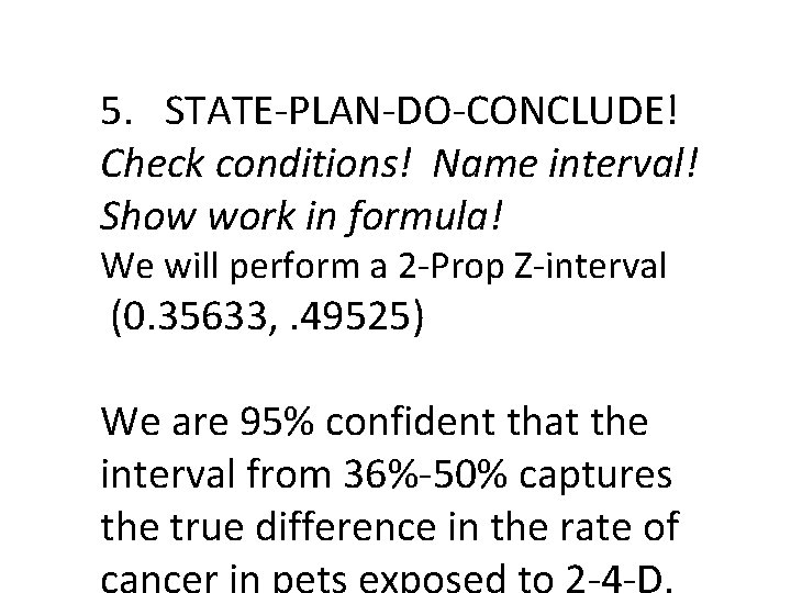
5. STATE-PLAN-DO-CONCLUDE! Check conditions! Name interval! Show work in formula! We will perform a 2 -Prop Z-interval (0. 35633, . 49525) We are 95% confident that the interval from 36%-50% captures the true difference in the rate of

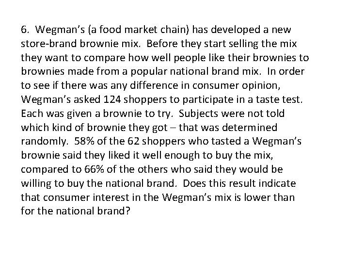
6. Wegman’s (a food market chain) has developed a new store-brand brownie mix. Before they start selling the mix they want to compare how well people like their brownies to brownies made from a popular national brand mix. In order to see if there was any difference in consumer opinion, Wegman’s asked 124 shoppers to participate in a taste test. Each was given a brownie to try. Subjects were not told which kind of brownie they got – that was determined randomly. 58% of the 62 shoppers who tasted a Wegman’s brownie said they liked it well enough to buy the mix, compared to 66% of the others who said they would be willing to buy the national brand. Does this result indicate that consumer interest in the Wegman’s mix is lower than for the national brand?

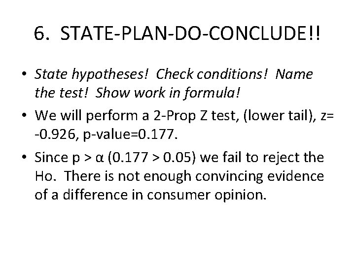
6. STATE-PLAN-DO-CONCLUDE!! • State hypotheses! Check conditions! Name the test! Show work in formula! • We will perform a 2 -Prop Z test, (lower tail), z= -0. 926, p-value=0. 177. • Since p > α (0. 177 > 0. 05) we fail to reject the Ho. There is not enough convincing evidence of a difference in consumer opinion.

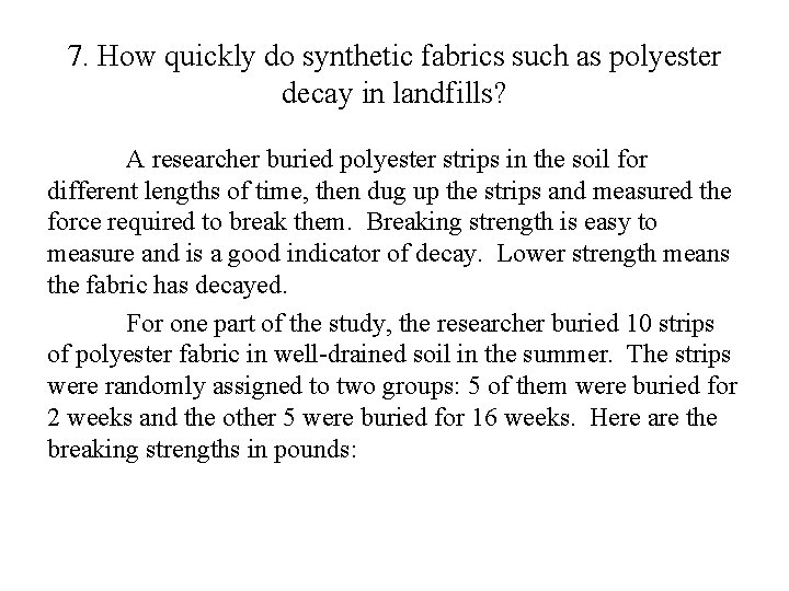
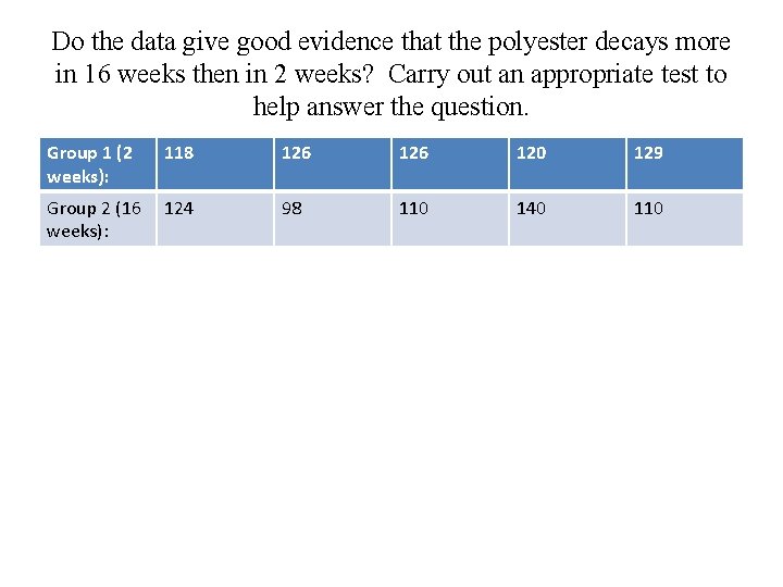
7. How quickly do synthetic fabrics such as polyester decay in landfills? A researcher buried polyester strips in the soil for different lengths of time, then dug up the strips and measured the force required to break them. Breaking strength is easy to measure and is a good indicator of decay. Lower strength means the fabric has decayed. For one part of the study, the researcher buried 10 strips of polyester fabric in well-drained soil in the summer. The strips were randomly assigned to two groups: 5 of them were buried for 2 weeks and the other 5 were buried for 16 weeks. Here are the breaking strengths in pounds:

Do the data give good evidence that the polyester decays more in 16 weeks then in 2 weeks? Carry out an appropriate test to help answer the question. Group 1 (2 weeks): 118 Group 2 (16 124 weeks): 126 120 129 98 110 140 110

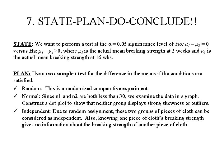
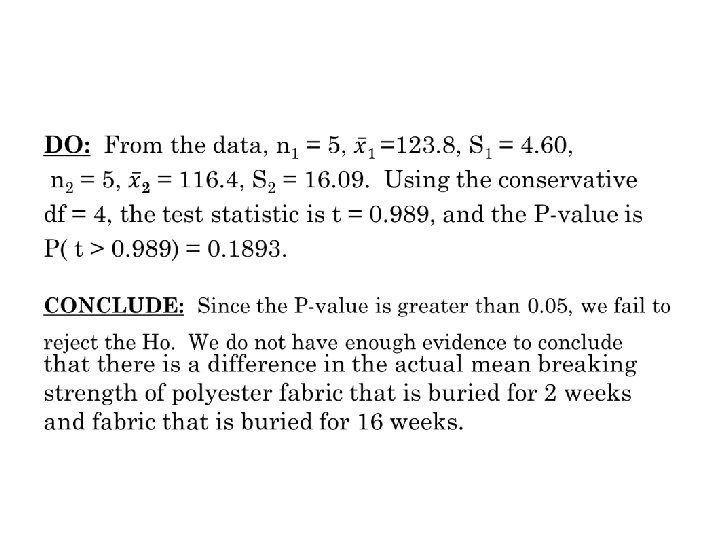
7. STATE-PLAN-DO-CONCLUDE!! STATE: We want to perform a test at the α = 0. 05 significance level of Ho: μ 1 – μ 2 = 0 versus Ha: μ 1 – μ 2 >0, where μ 1 is the actual mean breaking strength at 2 weeks and μ 2 is the actual mean breaking strength at 16 wks. PLAN: Use a two-sample t test for the difference in the means if the conditions are satisfied. ü Random: This is a randomized comparative experiment. ü Normal: Since n 1 and n 2 are both less than 30, we examine the data in a graph. Construct a dot plot to show that neither group displays strong skewness or outliers. ü Independent: Due to random assignment, these two groups of pieces of cloth can be considered as independent. Also, knowing one piece of cloth’s breaking strength gives no information about the breaking strength of another piece of cloth.

HOMEWORK! • Read and review Chapter 10! • To be collected on test day: --This review sheet, completed – Chapter 10 Review exercises, p. 661 -664, for extra credit – Finish Webassign!