CEDA Theory Session FMSP Stock Assessment Tools Training

CEDA Theory Session FMSP Stock Assessment Tools Training Workshop Mangalore College of Fisheries 20 th -24 th September 2004

What CEDA does The CEDA software analyses catch, effort and abundance data to provide estimates of: • • Unexploited or initial stock size (K or N 1) Catchability (q) or power of fishing Current stock size/biomass (performance indicator) MSY (reference point - DRP models only). CEDA also has a facility to project stock sizes into the future under various scenarios.

CEDA Theory - Contents Analysis of catch, effort and abundance data CEDA data requirements Models available in CEDA: No recruitment Indexed Recruitment models Deterministic Recruitment / Production (DRP) Models Choice of appropriate models Model outputs and use Guide to fitting models (Theory Session 2) Error Models Residual Plots Outliers Influential Points Sensitivity Analysis Confidence Limits and Bootstrapping Summary

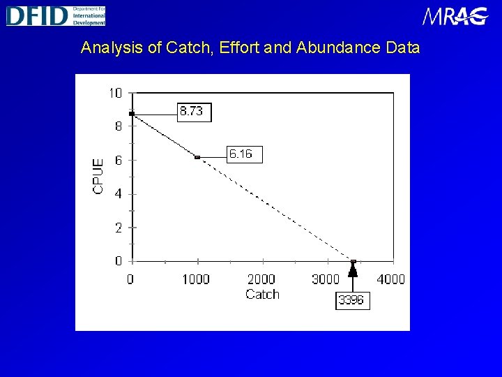
Analysis of Catch, Effort and Abundance Data The models used in CEDA are designed to mimic the changes over time (the dynamics) in the total numbers or total biomass of an exploited fish stock. For each model, it is assumed that you have historical data on the total catches that have been taken, and on an index of relative abundance (e. g. CPUE). Given these, using CEDA, you can then estimate the historical population abundances and the associated fishery parameters. You will also be able to predict how a stock will react to different future effort or catch scenarios and thus be able to manage and plan the fisheries better.

Analysis of Catch, Effort and Abundance Data

CEDA Data Requirements (1/2) All the models in CEDA assume that the data refers to a single discrete stock, i. e. a population without any significant immigration from that population or emigration to other population not covered by the data. Comprehensive record of total catch for the whole time period to be analysed, with no gaps. A “Good” relative index of population size or abundance. The two most common types of index are research survey data and commercial CPUE data. There can be advantages and disadvantages to both. .

CEDA Data Requirements (2/2) Research Survey Data Good measure of population size, but low sample size and low frequency therefore causing high variability. Commercial CPUE Cheap to collect, lower variability, but is it a “good” measure of population size?

Potential problems with CPUE data Way in which effort is measured. Target switching. Changes in fishing power. Sequential depletion.

CEDA Model Types of models available: 1. 1. No recruitment 2. 2. Indexed Recruitment 3. 3. Deterministic Recruitment / Production Models: • • Constant recruitment Schaefer production model Fox production model Pella-Tomlinson production model The correct choice of model is vital and depends on the pattern of recruitment to the fishery and the data available

No Recruitment Model These are typically used for within-season assessments of short-lived, annual species such as squid and shrimp. Also useful for the analysis of experimental fishing, where you fish for a short period in one location and assume that there was no recruitment during the period. Assumes that there is one pulse of recruitment at the start of the series and nothing after this point. (I. e. ‘no recruitment’ within the data set) Constant natural mortality (M) is assumed throughout. Requires catch and abundance index in numbers. (can use mean weight in each week to convert catch in weight)

Problems with the No Recruitment Model With the no recruitment model the assumption is made that the spatial distribution is constant. Therefore problems occur for “within-year” analyses where migration occurs, e. g. - Juveniles moving to / from nursery grounds - Adults moving to / from spawning - Migration of the adult stock This will affect the catchability or CPUE series, and make the estimates of population size unreliable.

Indexed recruitment model Typical of small pelagic species such as sardines and anchovies. Need an index of relative recruitment that is proportional to the number of recruits in each year. This is the only method in CEDA that can cope with substantial inter-annual variability in recruitment. How to get this index? - Larval or juvenile survey data Catch data from another fishery operating in the same area, but catching smaller animals Length-frequency data. Assumes constant M (Natural Mortality rate). Requires catches in numbers.

Problems with the indexed recruitment model The indexed recruitment model can sometimes produce unreliable estimates of population size, e. g. when: - The recruitment index is not a “good” measure of relative annual recruitment. - There is little annual variability in recruitment. It is possible to use an indirect estimate of recruitment such as a measure of upwelling, but this is not usually recommended.

Deterministic Production Models “Deterministic” - Describes a system whose time evolution can be predicted exactly. “Production” – In this case production refers to the net production in terms of yield after recruitment, growth, migration (into and out of the population) and natural mortality have been taken into account. Models assume constant carrying capacity (K) Two types - “Constant Recruitment” “Production Models”

Constant Recruitment Model First described by Allen (1966) with respect to whales. It has also been used for some reef fish species. Assumes that the stock started in deterministic equilibrium and that annual recruitment (in numbers) is constant and independent of stock size! This assumption may seem a little strange, but for many stocks it appears that recruitment declines only when the adult stock has been reduced to rather low levels (e. g. around 20% of unexploited levels). The method is not suitable for use when there is substantial interannual variation in recruitment.

Production Models Deterministic Production Models work on the basis that the net change in biomass of a population from one year to the next is a result of: • the catch taken during the current year, and • the “stock production” during the current year. The stock production combines the effects of recruitment to the population, growth and natural mortality, and it is assumed to be a deterministic function of current or recent stock sizes.

Production Models Three production models are included in CEDA: Schaefer Production Model Fox Production Model Pella-Tomlinson Production Model

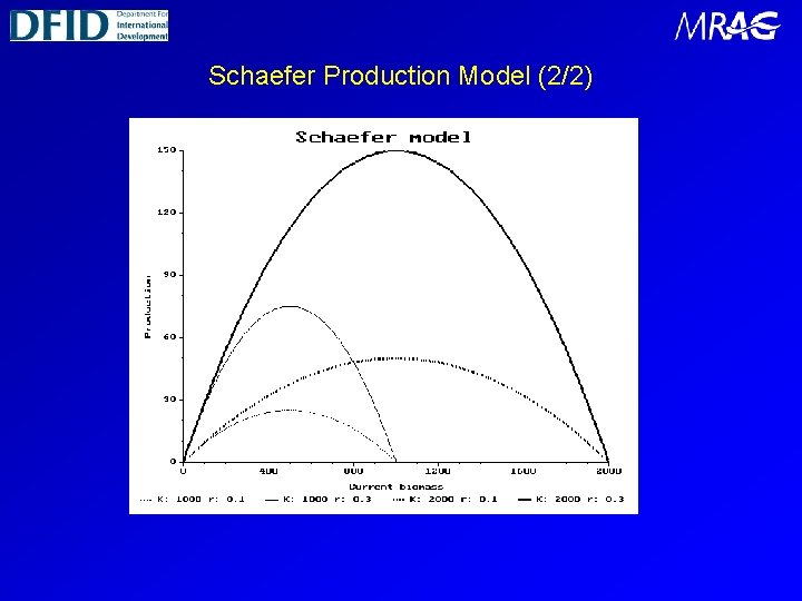
Schaefer Production Model (1/2) The Schaefer production model (Schaefer, 1954) assumes that there is a symmetrical relationship between stock size and production (and yield), which is a function of the unexploited population size (or carrying capacity) K, and the intrinsic growth rate r. For Schaefer models, the sustainable yield curves are symmetrical and they all have a maximum ( the maximum sustainable yield, or MSY) which occurs at a biomass of K/2. In order to obtain reliable estimates of r and K, data must be available for a wide range of stock sizes (giving good ‘contrast’)

Schaefer Production Model (2/2)

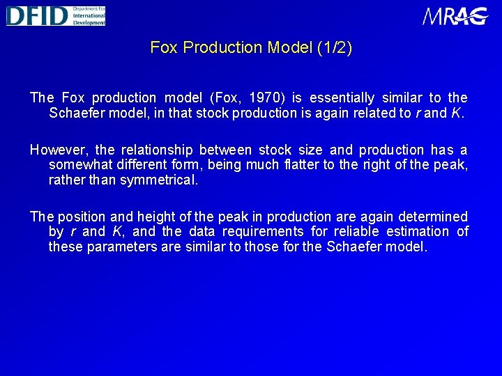
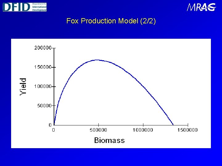
Fox Production Model (1/2) The Fox production model (Fox, 1970) is essentially similar to the Schaefer model, in that stock production is again related to r and K. However, the relationship between stock size and production has a somewhat different form, being much flatter to the right of the peak, rather than symmetrical. The position and height of the peak in production are again determined by r and K, and the data requirements for reliable estimation of these parameters are similar to those for the Schaefer model.

Fox Production Model (2/2)

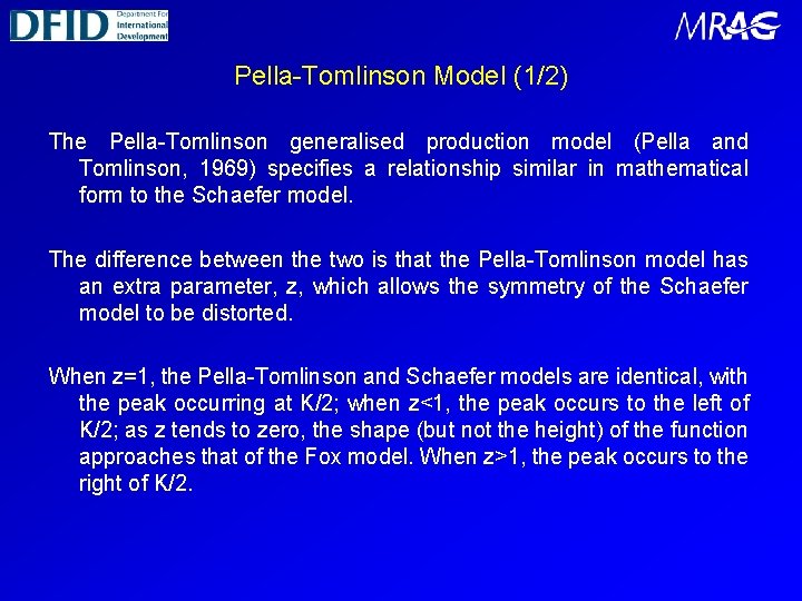
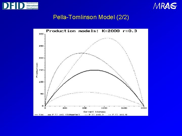
Pella-Tomlinson Model (1/2) The Pella-Tomlinson generalised production model (Pella and Tomlinson, 1969) specifies a relationship similar in mathematical form to the Schaefer model. The difference between the two is that the Pella-Tomlinson model has an extra parameter, z, which allows the symmetry of the Schaefer model to be distorted. When z=1, the Pella-Tomlinson and Schaefer models are identical, with the peak occurring at K/2; when z<1, the peak occurs to the left of K/2; as z tends to zero, the shape (but not the height) of the function approaches that of the Fox model. When z>1, the peak occurs to the right of K/2.

Pella-Tomlinson Model (2/2)

Time Lags in Production Models Often fish do not recruit into the fishery at age 0. Many fish have a long juvenile phase where they are not fished as part of the exploited stock. This means that the effects of a much lower (or higher) adult stock size in one year, in terms of subsequent lower (or higher) recruitment, may not be apparent for a number of years. To account for these cases, CEDA allows you to incorporate a time lag “L” into the DRP models, linking biomass production with the stock size L years ago. NOTE, however, that recruitment is only one part of production, the other parts of which definitely happen during the current year. Normally, we recommend time lags are not used.

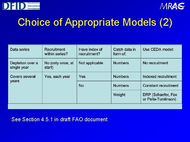
Choice of Appropriate Models Often, only one of the six models described above will be suitable for the type of data available. If you have weekly data from a species without recruitment, then use the norecruitment model. If you have annual data with a recruitment index, then use the indexed recruitment model. You may also want to try a production model. If you only have annual catch and abundance data in weight, then you will have to use a production model. There are two main situations in which you have a choice over the model Constant recruitment model vs DRP model Three alternative DRP models

Choice of Appropriate Models (2) See Section 4. 5. 1 in draft FAO document

Choice of Timescale If you have monthly data collected over a number of years, then would normally aggregate over 12 month periods. However, if noticeable seasonality in catch rates, should still aggregate catch data over 12 month period, but only use CPUE data from months with the highest catch rates. Remember years do not necessarily start in January!

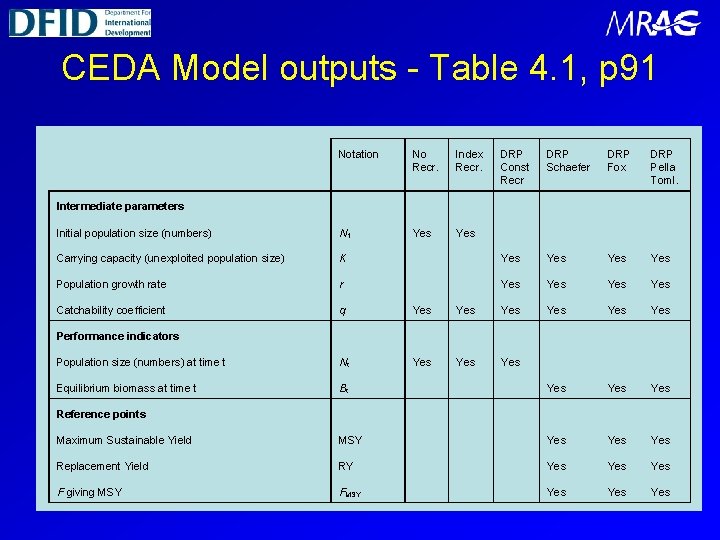
CEDA Model outputs - Table 4. 1, p 91 Notation No Recr. Index Recr. DRP Const Recr DRP Schaefer DRP Fox DRP Pella Toml. Initial population size (numbers) N 1 Yes Carrying capacity (unexploited population size) K Yes Yes Population growth rate r Yes Yes Catchability coefficient q Yes Yes Yes Population size (numbers) at time t Nt Yes Yes Equilibrium biomass at time t Bt Yes Yes Maximum Sustainable Yield MSY Yes Yes Replacement Yield RY Yes Yes F giving MSY FMSY Yes Yes Intermediate parameters Performance indicators Reference points

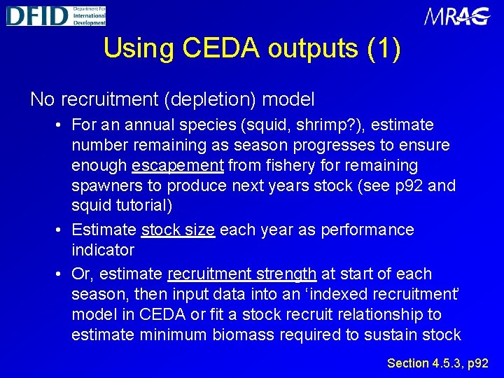
Using CEDA outputs (1) No recruitment (depletion) model • For an annual species (squid, shrimp? ), estimate number remaining as season progresses to ensure enough escapement from fishery for remaining spawners to produce next years stock (see p 92 and squid tutorial) • Estimate stock size each year as performance indicator • Or, estimate recruitment strength at start of each season, then input data into an ‘indexed recruitment’ model in CEDA or fit a stock recruit relationship to estimate minimum biomass required to sustain stock Section 4. 5. 3, p 92

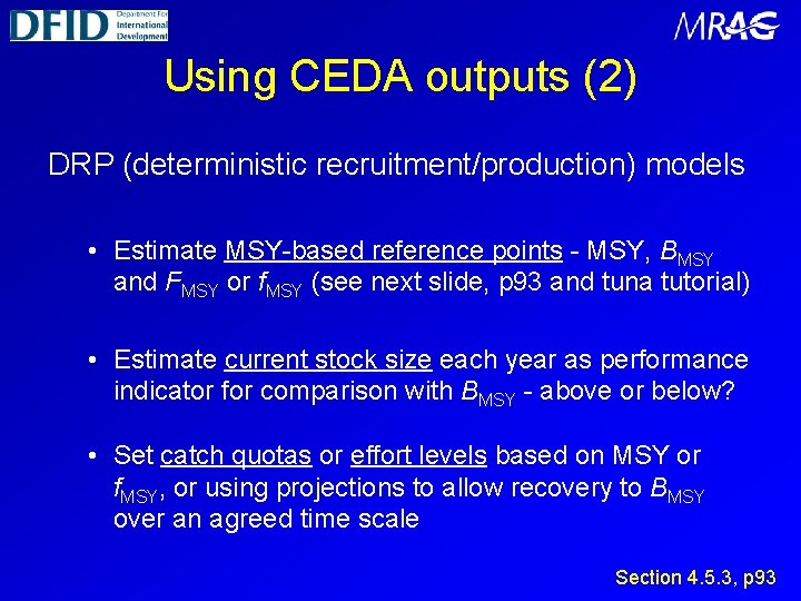
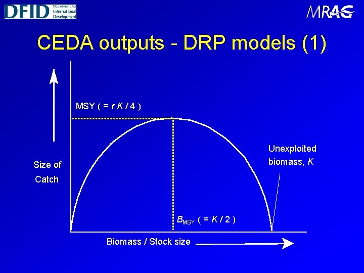
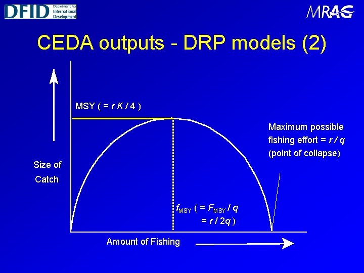
Using CEDA outputs (2) DRP (deterministic recruitment/production) models • Estimate MSY-based reference points - MSY, BMSY and FMSY or f. MSY (see next slide, p 93 and tuna tutorial) • Estimate current stock size each year as performance indicator for comparison with BMSY - above or below? • Set catch quotas or effort levels based on MSY or f. MSY, or using projections to allow recovery to BMSY over an agreed time scale Section 4. 5. 3, p 93

CEDA outputs - DRP models (1) MSY ( = r K / 4 ) Unexploited biomass, K Size of Catch BMSY ( = K / 2 ) Biomass / Stock size

CEDA outputs - DRP models (2) MSY ( = r K / 4 ) Maximum possible fishing effort = r / q (point of collapse) Size of Catch f. MSY ( = FMSY / q = r / 2 q ) Amount of Fishing

CEDA Theory Part 2 Guide to Fitting Models Error Models Residual Plots Outliers Influential Points Sensitivity Analysis Confidence Intervals

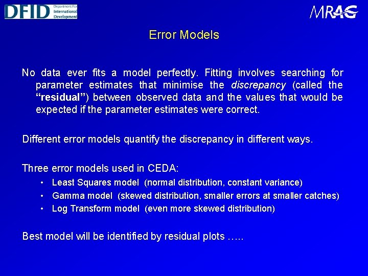
Error Models No data ever fits a model perfectly. Fitting involves searching for parameter estimates that minimise the discrepancy (called the “residual”) between observed data and the values that would be expected if the parameter estimates were correct. Different error models quantify the discrepancy in different ways. Three error models used in CEDA: • Least Squares model (normal distribution, constant variance) • Gamma model (skewed distribution, smaller errors at smaller catches) • Log Transform model (even more skewed distribution) Best model will be identified by residual plots …. .

Residual Plots (1/4) Once you have tried a particular fit, you will obtain both parameter estimates and a range of “diagnostics”, which should help you to determine whether your fit was good. The most important diagnostics are simply the graphs of observed and expected values of catch and CPUE. Looking at these will soon reveal whether you have a reasonably good fit. The residual plots are closely related to the catch graph, and their purpose is to enable model assumptions to be checked. Two residual plots are available: • residuals plotted against the expected catch; • residuals plotted against time.

Residual Plots (2/4) The figure below is an example of a good residual plot. The points observed are scattered evenly in a horizontal band above and below the zero residual line and over time.

Residual Plots (3/4) The following is an example of a bad residual plot. This curved shape to the plot shows that the population model used does not fit the data correctly. Bad plots can be identified by trends or runs of individual points on either side of the zero residual.

Residual Plots (4/4) Another bad plot. Here the shape shown by the points is not evenly distributed. Here smaller residuals appear at low catch values and higher residuals at higher values. This type of plot can occur when the wrong error models have been used.

Outliers (1/4) An outlier in a data set fitted with a particular model is an observation that would be extremely unlikely to occur under the best fitting model. The main way of detecting outliers is by examining the residual plots. An outlier is a point that lies a "long way" from the x-axis (or 0. 5 line on a percentile plot) relative to the other points. The definition of a "long way" depends on the probability of accidentally labeling a perfectly good data point as an outlier. The occurrence of an outlier indicates that there is probably a fault with either the model or the data.

Outliers (2/4) An example of a outlier in a CPUE series is shown below. The very high CPUE shown at t=7 is also shown in the outlier in the residual plot. The “error” here in the data was down to poor data entry with the effort entered being ten times the amount that was actually recorded.

Outliers (3/4) Any apparent outliers should be subjected to further scrutiny. If an outlier occurs with a model that seems to fit the other data well, the first task is to investigate the offending point or points. The problem could be caused by unusual conditions at that time or by measurement errors in the abundance index, catch data, recruitment index, or even the mean weight.

Outliers (4/4) If conditions were anomalous at that time (e. g. unusual sea temperature), then the point may be excluded from analysis (when you do this, you should also check the other data for a similar circumstance; any other similarly anomalous points should be excluded as well, even if they do not appear to be outliers). Outliers may disappear under different error model If an outlier still exists and no good reason exists for it’s removal then sensitivity analysis can be carried out with reference to that point.

Influential Points (1/2) Influential points are those whose presence or absence make a large difference to the results. Influential points tend usually, but not invariably, to lie near the extremes of the data set, i. e. near the lowest and highest stock sizes. Influential points can often be identified from plots of residuals against expected catches: they will be points corresponding to isolated large or small expected catches, usually with small residuals. If you suspect that a point is influential, you can easily check by toggling it out and seeing if the parameter estimates change substantially.

Influential Points (2/2) The data for an influential point should be carefully scrutinized, just as for a potential outlier. If there are serious data problems, then the point could be dropped from subsequent analysis. As for outliers you must have very good reasons to exclude the point from analysis. If no good reason exists, then sensitivity analysis should be used. What are the effects of including and excluding the point? It is definitely wrong to exclude an influential point and then "forget" about it, as one might for an outlier; you will bias the results and will dramatically reduce the precision of your estimates.

Sensitivity Analysis Investigate the effect of varying the model assumptions when you are uncertain about which is correct. It is better to be honest about the uncertainty in one's results than it is to be wrong! Try different assumptions: - Different models - Different data - Different error models - Including / excluding influential points from the model - Different values for user-supplied parameters (e. g. M) Present results of all sensitivity analyses to decision makers so that the real uncertainty in the results will be clear

Confidence Intervals Should not only look at point estimates, need to also consider confidence intervals (CI’s), in addition to sensitivity tests. A CI of a given size, e. g. 95%, is the probability that the interval contains the true value. Should form management decisions based on CI’s, rather than point estimates alone. (Remember precautionary reference points) Estimate CI’s as part of sensitivity analysis. Comparing two point values may show them to be quite different but the overlap of their CI’s may be very similar. Estimate CI’s by bootstrapping….

Bootstrapping uses the set of discrepancies between observed and expected values in the original data to simulate new data sets, or “re -samples”. For each re-sampled data set, the parameter estimation procedure is repeated. Bootstrapping will show any skewness in the estimates, but care should be taken with any values appearing at 0 and as these may be false values caused by repeated selection on a particular (“wrong”) value. The problem with bootstrapping is that it can be a slow process. Less of a problem now with higher powered computers but be wary on older machines.

Summary (CEDA Theory) What have we covered? Analysis of catch, effort and abundance data CEDA data requirements Models available in CEDA • No recruitment models • Constant recruitment models • Deterministic Recruitment / Production (DRP) Models Choice of appropriate models Use of CEDA outputs Guide to fitting models - residual plots etc