Application of inverse methods to constrain methane emissions

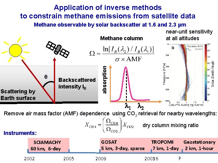
Application of inverse methods to constrain methane emissions from satellite data Scattering by Earth surface Backscattered intensity IB absorption Methane observable by solar backscatter at 1. 6 and 2. 3 µm near-unit sensitivity at all altitudes Methane column l 1 l 2 Remove air mass factor (AMF) dependence using CO 2 retrieval for nearby wavelengths: dry column mixing ratio Instruments: GOSAT 5 km, 3 -day, sparse SCIAMACHY 60 km, 6 -day 2002 2005 2009 TROPOMI Geostationary 7 km, 1 -day 2 km, 1 -hour 20016 ?

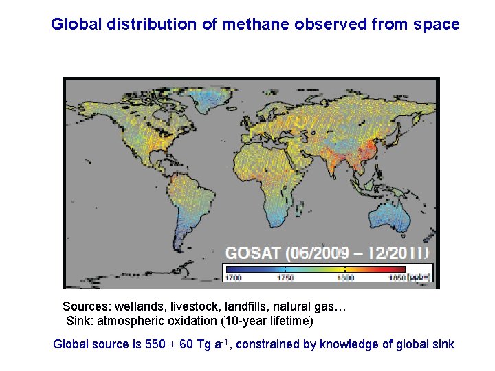
Global distribution of methane observed from space Sources: wetlands, livestock, landfills, natural gas… Sink: atmospheric oxidation (10 -year lifetime) Global source is 550 60 Tg a-1, constrained by knowledge of global sink

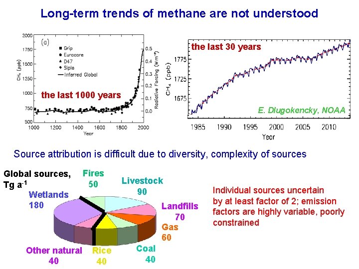
Long-term trends of methane are not understood the last 30 years the last 1000 years E. Dlugokencky, NOAA Source attribution is difficult due to diversity, complexity of sources Global sources, Tg a-1 Wetlands 180 Other natural 40 Fires 50 Livestock 90 Landfills 70 Gas 60 Rice 40 Coal 40 Individual sources uncertain by at least factor of 2; emission factors are highly variable, poorly constrained

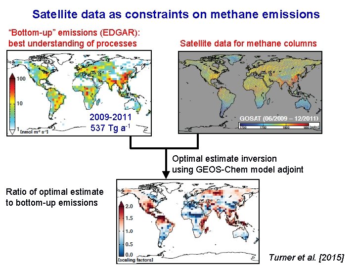
Satellite data as constraints on methane emissions “Bottom-up” emissions (EDGAR): best understanding of processes Satellite data for methane columns 2009 -2011 537 Tg a-1 Optimal estimate inversion using GEOS-Chem model adjoint Ratio of optimal estimate to bottom-up emissions Turner et al. [2015]

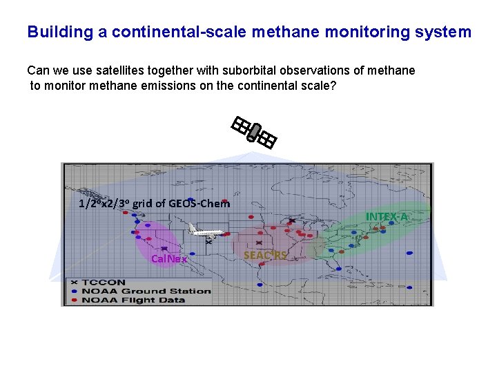
Building a continental-scale methane monitoring system Can we use satellites together with suborbital observations of methane to monitor methane emissions on the continental scale? 1/2 ox 2/3 o grid of GEOS-Chem Cal. Nex INTEX-A SEAC 4 RS

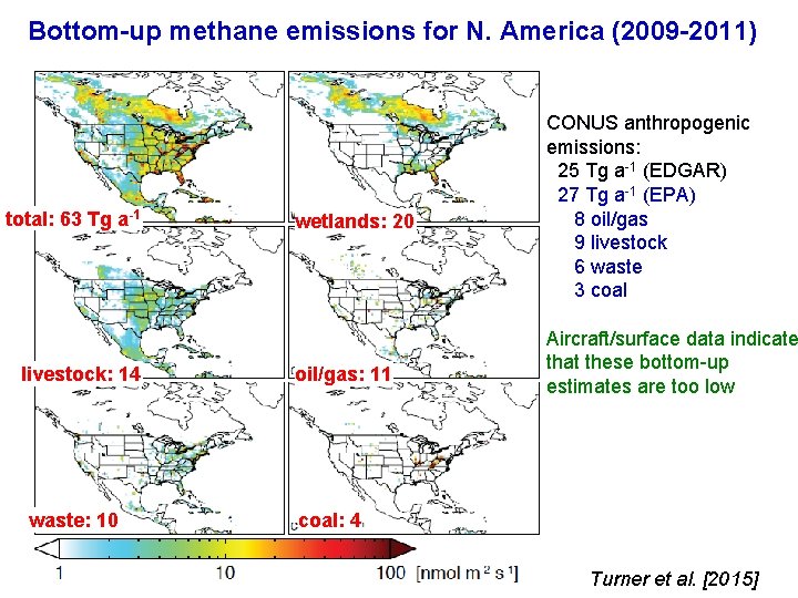
Bottom-up methane emissions for N. America (2009 -2011) total: 63 Tg a-1 livestock: 14 waste: 10 wetlands: 20 oil/gas: 11 CONUS anthropogenic emissions: 25 Tg a-1 (EDGAR) 27 Tg a-1 (EPA) 8 oil/gas 9 livestock 6 waste 3 coal Aircraft/surface data indicate that these bottom-up estimates are too low coal: 4 Turner et al. [2015]

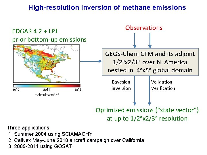
High-resolution inversion of methane emissions EDGAR 4. 2 + LPJ prior bottom-up emissions Observations GEOS-Chem CTM and its adjoint 1/2 ox 2/3 o over N. America nested in 4 ox 5 o global domain Bayesian inversion Validation Verification Optimized emissions (“state vector”) at up to 1/2 ox 2/3 o resolution Three applications: 1. Summer 2004 using SCIAMACHY 2. Cal. Nex May-June 2010 aircraft campaign over California 3. 2009 -2011 using GOSAT

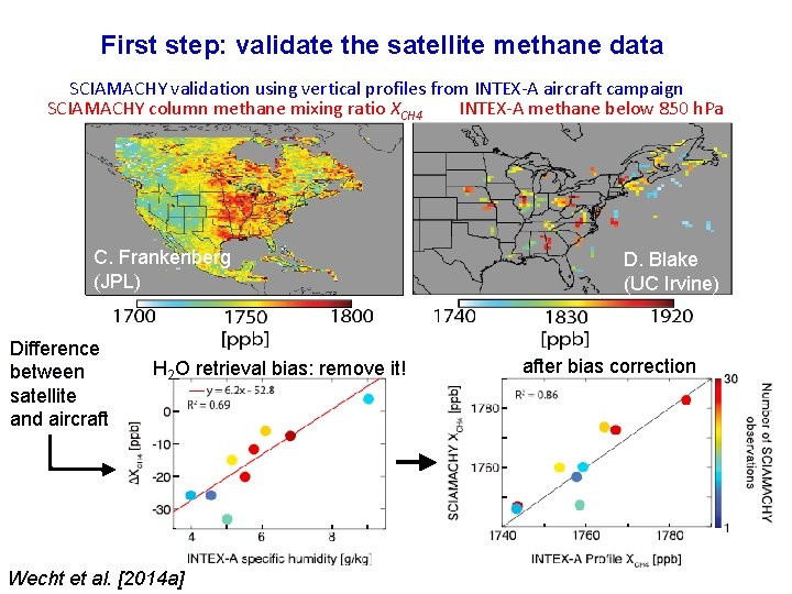
First step: validate the satellite methane data SCIAMACHY validation using vertical profiles from INTEX-A aircraft campaign SCIAMACHY column methane mixing ratio XCH 4 INTEX-A methane below 850 h. Pa Frankenberg C. C. Frankenberg (JPL) Difference between satellite and aircraft H 2 O retrieval bias: remove it! Wecht et al. [2014 a] D. Blake (UC Irvine) after bias correction

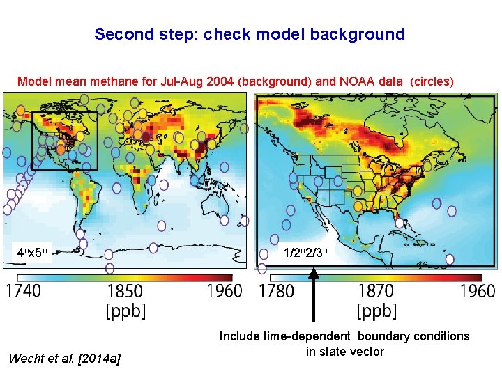
Second step: check model background Model mean methane for Jul-Aug 2004 (background) and NOAA data (circles) 4 ox 5 o Wecht et al. [2014 a] 1/2 o 2/3 o Include time-dependent boundary conditions in state vector

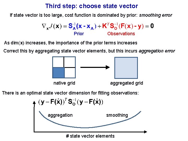
Third step: choose state vector If state vector is too large, cost function is dominated by prior: smoothing error Prior Observations As dim(x) increases, the importance of the prior terms increases Correct this by aggregating state vector elements, but this incurs aggregation error native grid aggregated grid There is an optimal state vector dimension for fitting observations: aggregation smoothing # state vector elements

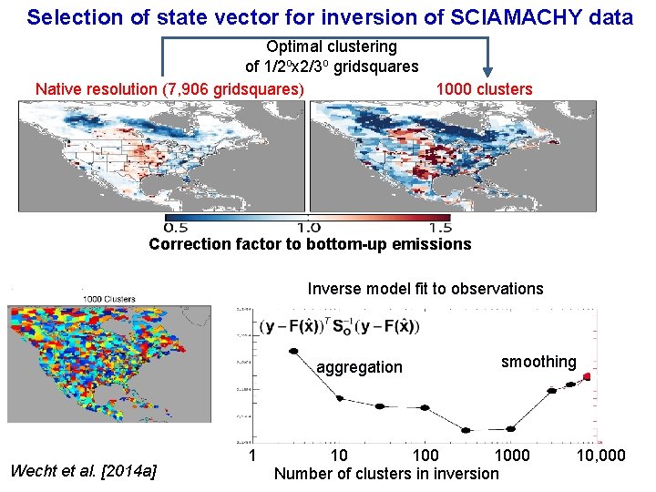
Selection of state vector for inversion of SCIAMACHY data Optimal clustering of 1/2 ox 2/3 o gridsquares Native resolution (7, 906 gridsquares) 1000 clusters Inverse model fit to observations 34 aggregation smoothing 28 Wecht et al. [2014 a] 1 10 1000 Number of clusters in inversion 10, 000 Optimized US emissions (Tg a-1) Correction factor to bottom-up emissions

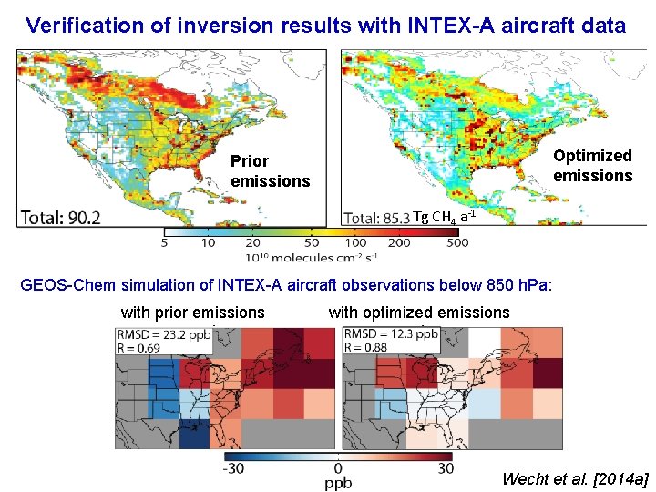
Verification of inversion results with INTEX-A aircraft data Optimized emissions Prior emissions Tg CH 4 a-1 GEOS-Chem simulation of INTEX-A aircraft observations below 850 h. Pa: with prior emissions with optimized emissions Wecht et al. [2014 a]

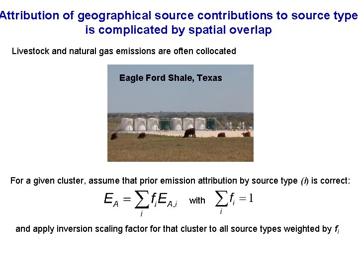
Attribution of geographical source contributions to source type is complicated by spatial overlap Livestock and natural gas emissions are often collocated Eagle Ford Shale, Texas For a given cluster, assume that prior emission attribution by source type (i) is correct: with and apply inversion scaling factor for that cluster to all source types weighted by fi

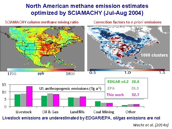
North American methane emission estimates optimized by SCIAMACHY (Jul-Aug 2004) SCIAMACHY column methane mixing ratio Correction factors to a priori emissions 1000 clusters 1700 15 10 5 ppb 1800 EDGAR v 4. 2 26. 6 US anthropogenic emissions (Tg a-1) EPA 28. 3 This work 32. 7 0 Livestock Oil & Gas Landfills Coal Mining Other Livestock emissions are underestimated by EDGAR/EPA, oil/gas emissions are not Wecht et al. [2014 a]

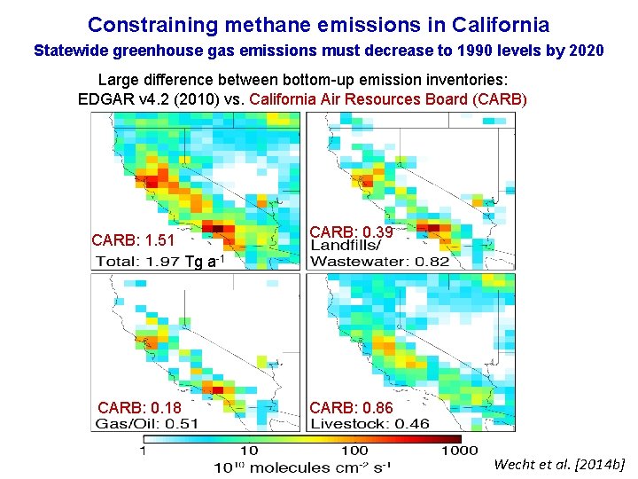
Constraining methane emissions in California Statewide greenhouse gas emissions must decrease to 1990 levels by 2020 Large difference between bottom-up emission inventories: EDGAR v 4. 2 (2010) vs. California Air Resources Board (CARB) CARB: 0. 39 CARB: 1. 51 Tg a-1 CARB: 0. 18 CARB: 0. 86 Wecht et al. [2014 b]

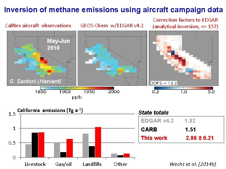
Inversion of methane emissions using aircraft campaign data Cal. Nex aircraft observations GEOS-Chem w/EDGAR v 4. 2 Correction factors to EDGAR (analytical inversion, n= 157) May-Jun 2010 G. Santoni (Harvard) 1. 5 California emissions (Tg a-1) State totals EDGAR v 4. 2 1 0. 5 0 Livestock Gas/oil Landfills Other 1. 92 CARB 1. 51 This work 2. 86 ± 0. 21 Wecht et al. [2014 b]

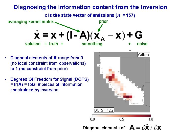
Diagnosing the information content from the inversion x is the state vector of emissions (n = 157) prior averaging kernel matrix solution = truth + smoothing • Diagonal elements of A range from 0 (no local constraint from observations) to 1 (no constraint from prior) • Degrees Of Freedom for Signal (DOFS) = tr(A) = total # pieces of information constrained by inversion Diagonal elements of + noise

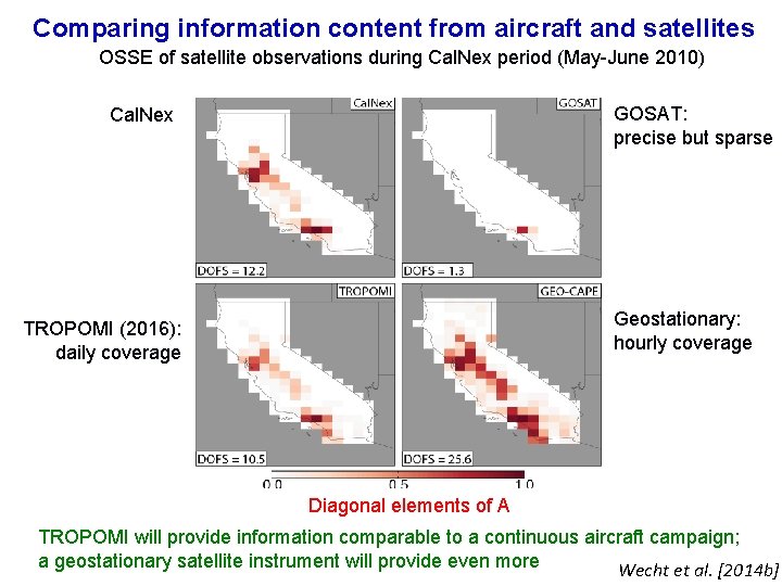
Comparing information content from aircraft and satellites OSSE of satellite observations during Cal. Nex period (May-June 2010) GOSAT: precise but sparse Cal. Nex Geostationary: hourly coverage TROPOMI (2016): daily coverage Diagonal elements of A TROPOMI will provide information comparable to a continuous aircraft campaign; a geostationary satellite instrument will provide even more Wecht et al. [2014 b]

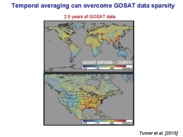
Temporal averaging can overcome GOSAT data sparsity 2. 5 years of GOSAT data Turner et al. [2015]

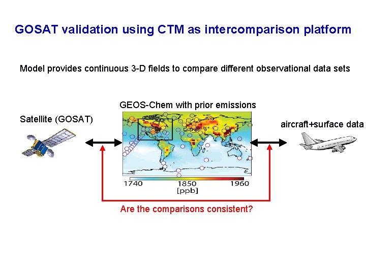
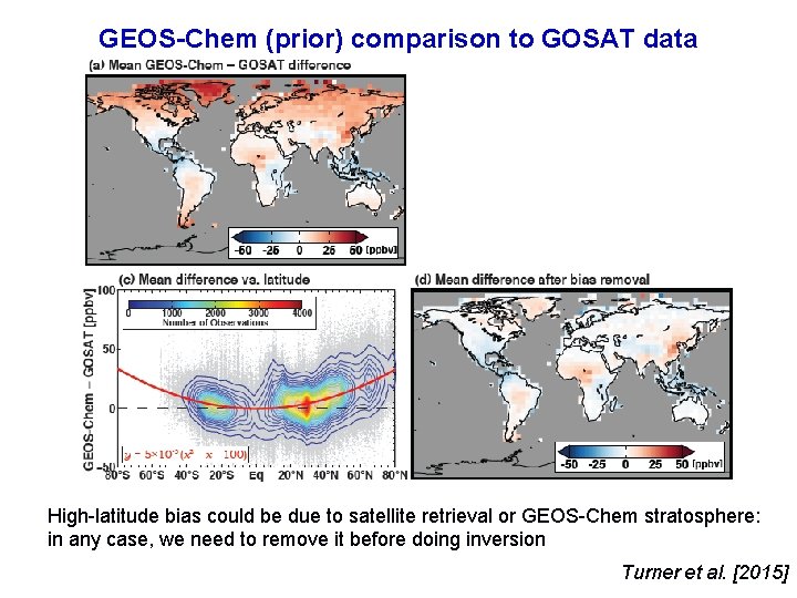
GOSAT validation using CTM as intercomparison platform Model provides continuous 3 -D fields to compare different observational data sets GEOS-Chem with prior emissions Satellite (GOSAT) aircraft+surface data Are the comparisons consistent?

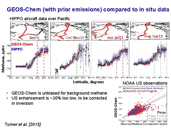
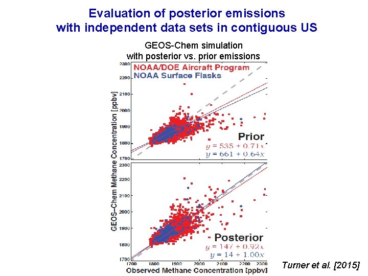
GEOS-Chem (with prior emissions) compared to in situ data HIPPO aircraft data over Pacific Methane, ppbv Jan 09 Oct-Nov 09 Jun-Jul 11 Aug-Sep 11 GEOS-Chem HIPPO Latitude, degrees Turner et al. [2015] GEOS-Chem • GEOS-Chem is unbiased for background methane • US enhancement is ~30% too low, to be corrected in inversion NOAA US observations

GEOS-Chem (prior) comparison to GOSAT data High-latitude bias could be due to satellite retrieval or GEOS-Chem stratosphere: in any case, we need to remove it before doing inversion Turner et al. [2015]

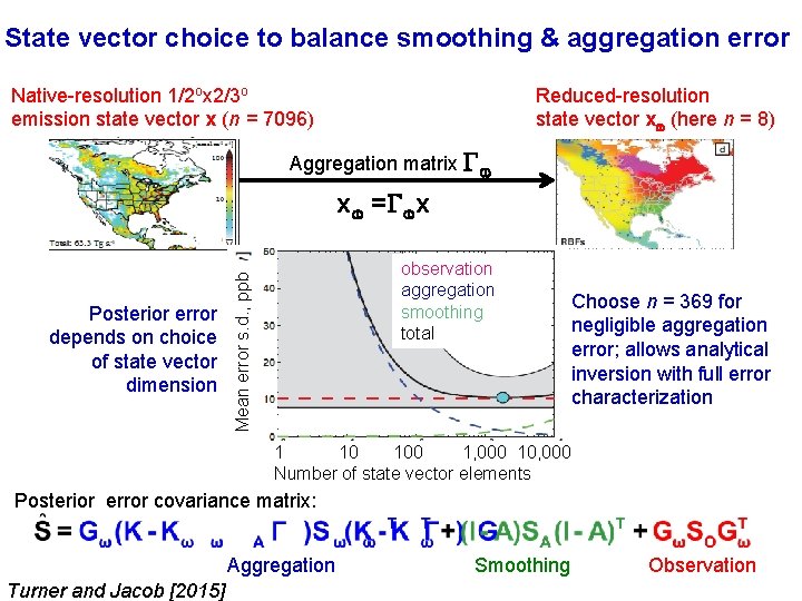
State vector choice to balance smoothing & aggregation error Native-resolution 1/2 ox 2/3 o emission state vector x (n = 7096) Reduced-resolution state vector x (here n = 8) Aggregation matrix x = x Mean error s. d. , ppb Posterior error depends on choice of state vector dimension observation aggregation smoothing total Choose n = 369 for negligible aggregation error; allows analytical inversion with full error characterization 1 10 100 1, 000 10, 000 Number of state vector elements Posterior error covariance matrix: Aggregation Turner and Jacob [2015] Smoothing Observation

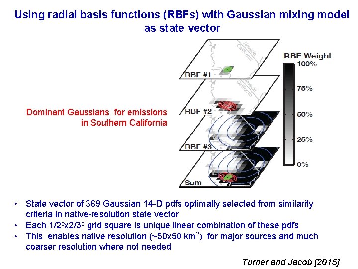
Using radial basis functions (RBFs) with Gaussian mixing model as state vector Dominant Gaussians for emissions in Southern California • State vector of 369 Gaussian 14 -D pdfs optimally selected from similarity criteria in native-resolution state vector • Each 1/2 ox 2/3 o grid square is unique linear combination of these pdfs • This enables native resolution (~50 x 50 km 2) for major sources and much coarser resolution where not needed Turner and Jacob [2015]

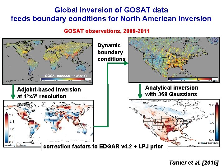
Global inversion of GOSAT data feeds boundary conditions for North American inversion GOSAT observations, 2009 -2011 Dynamic boundary conditions Adjoint-based inversion at 4 ox 5 o resolution Analytical inversion with 369 Gaussians correction factors to EDGAR v 4. 2 + LPJ prior Turner et al. [2015]

Averaging kernel sensitivities and inversion results Turner et al. [2015]

Evaluation of posterior emissions with independent data sets in contiguous US GEOS-Chem simulation Comparison of California results with posterior vs. to prior emissions previous inversions of Cal. Nex data (Los Angeles) Turner et al. [2015]

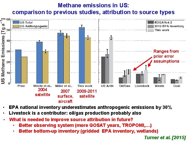
Methane emissions in US: comparison to previous studies, attribution to source types Ranges from prior error assumptions 2004 satellite 2007 2009 -2011 surface, satellite aircraft • EPA national inventory underestimates anthropogenic emissions by 30% • Livestock is a contributor: oil/gas production probably also • What is needed to improve source attribution in future? • Better observing system (more GOSAT years, TROPOMI, …) • Better bottom-up inventory (gridded EPA inventory, wetlands) Turner et al. [2015]

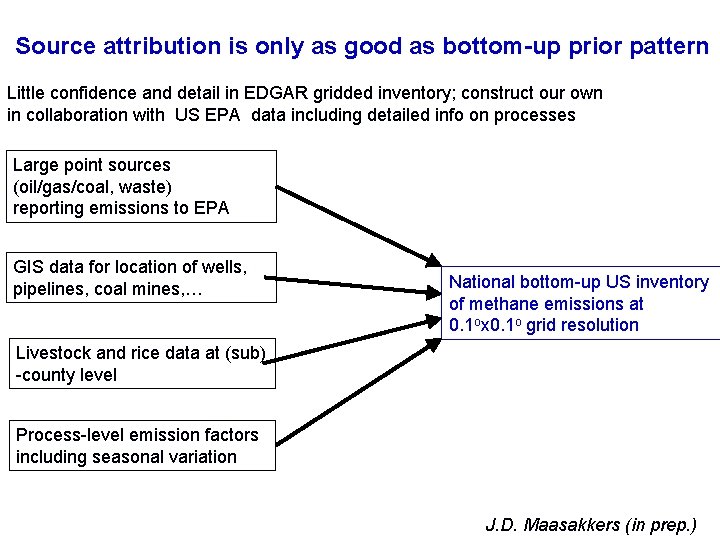
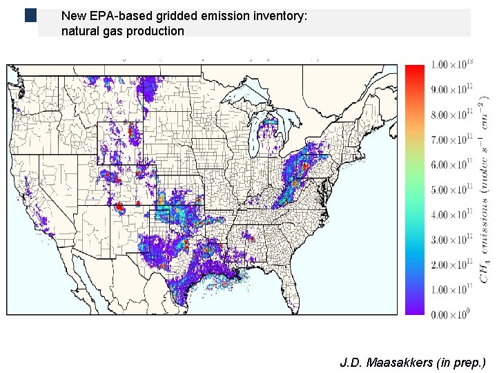
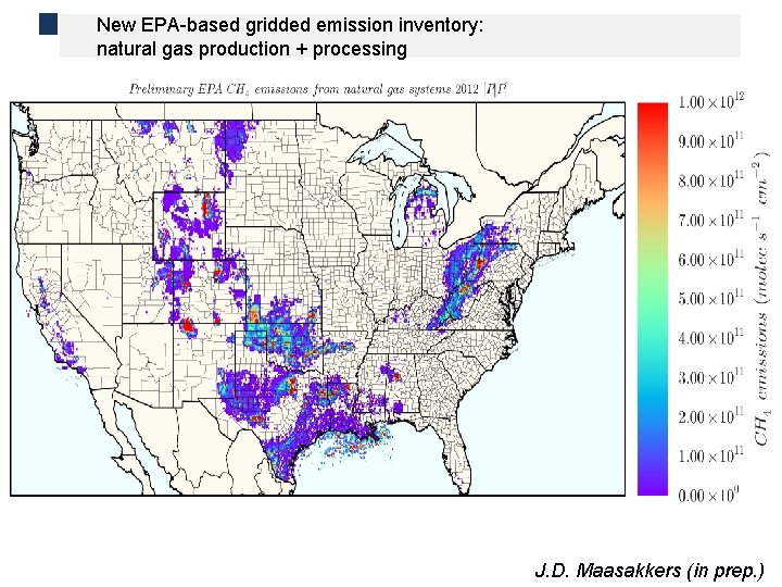
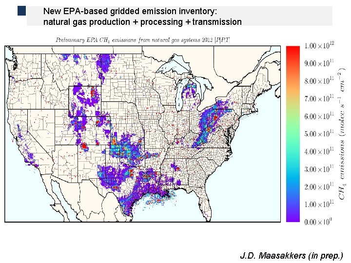
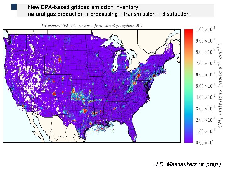
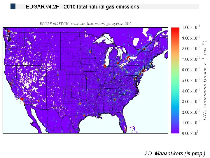
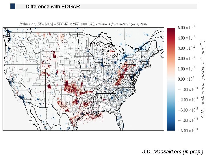
Source attribution is only as good as bottom-up prior pattern Little confidence and detail in EDGAR gridded inventory; construct our own in collaboration with US EPA data including detailed info on processes Large point sources (oil/gas/coal, waste) reporting emissions to EPA GIS data for location of wells, pipelines, coal mines, … National bottom-up US inventory of methane emissions at 0. 1 ox 0. 1 o grid resolution Livestock and rice data at (sub) -county level Process-level emission factors including seasonal variation J. D. Maasakkers (in prep. )

New EPA-based gridded emission inventory: natural gas production J. D. Maasakkers (in prep. )

Natural gas processing New EPA-based gridded emission inventory: natural gas production + processing J. D. Maasakkers (in prep. )

Natural gas transmission New EPA-based gridded emission inventory: natural gas production + processing + transmission J. D. Maasakkers (in prep. )

Total EPA-based natural gas: gridded production + processing + transmission + distribution New emission inventory: natural gas production + processing + transmission + distribution J. D. Maasakkers (in prep. )

EDGAR v 4. 2 FT 2010 total natural gas emissions J. D. Maasakkers (in prep. )

Difference with EDGAR J. D. Maasakkers (in prep. )