Analytical Loop Closure Applications to Loop Modeling Chaok

Analytical Loop Closure & Applications to Loop Modeling

Chaok Seok, Evangelos Coutsias, Matthew Jacobson, and Ken Dill Dept of Pharmaceutical Chemistry, UCSF and Dept of Mathematics and Statistics, Univ. of New Mexico

Abstract We consider the problem of loop closure, i. e. , of finding the ensemble of possible backbone structures of a chain molecule that is geometrically consistent with preceding and following parts of the chain whose structures are given. We provide a simple intuitive view and derivation of a 16 th degree polynomial equation for the case in which each of the three pairs of torsional axes has a common point. Our method generalizes previous work on analytical loop closure in that the torsion angles need not be consecutive, and any rigid intervening segments are allowed between the free torsions. We give applications to important problems. First, we show that this algorithm can be efficiently combined with an existing loop construction algorithm to sample protein loops longer than three residues. Second, we show that Monte Carlo minimization is made several fold more efficient by employing the local moves generated by the loop closure algorithm.

1 r 69: Res 9 -19 alternative backbone configurations

Representation of Loop Structures In the original frame In the new frame

New View of Loop Closure Old View New View 6 rotations / 6 constraints 3 rotations / 3 constraints

Crank Follower Two-revolute, two-spheric-pair mechanism

The 4 -bar spherical linkage

y d x z

z y R 1 R 2 1 2 x L 1 L 2 4 3 A complete cycle through the allowed values for j (dihedral (R 1, R 2) -(L 1, R 1) )and y (dihedral (R 1, R 2)-(L 2, R 2))

t a =. 35*p r 1=. 81=r 2

Derivation of a 16 th Degree Polynomial for the 6 -angle Loop Closure 2 ri-1 ·ri = cos i gives Pi(ui-1, ui) =j, k=0 pjk ui-1 j uik , where ui = tan( i/2). Using the method of resultants, the three biquadratic equations P 1(u 3, u 1), P 2(u 1, u 2), and P 3(u 2, u 3) are reduced to a polynomial in u 3, r 16 R 16(u 3) = rj u 3 j j=0 r 1 2

Method of resultants gives an equivalent 16 th degree polynomial for a single variable Numerical evidence that at most 8 real solutions exist. Must be related to parameter values: the similar problem of the 6 R linkage in a multijointed robot arm is known to possess 16 solutions for certain ranges of parameter values (Wampler and Morgan ’ 87; Lee and Liang ‘’ 89).

The Minkowski sum of three squares, of side a, b, c resp. Here a=2 x, b=2 y, c=2 z are the sizes of three scaled Newton polytopes for the three biquadratics

There at most 16 solutions: from first principles By the Bernstein-Kushnirenko-Khovanski theorem the total number of isolated solutions cannot exceed the mixed volume of the Minkowski sum of the Newton Polytopes of the consitutive polynomial components. That is, the number 16 is generic for this problem.

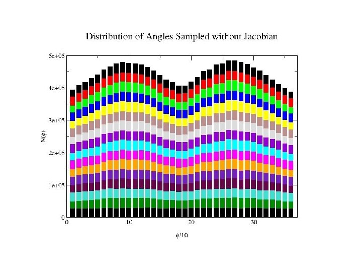
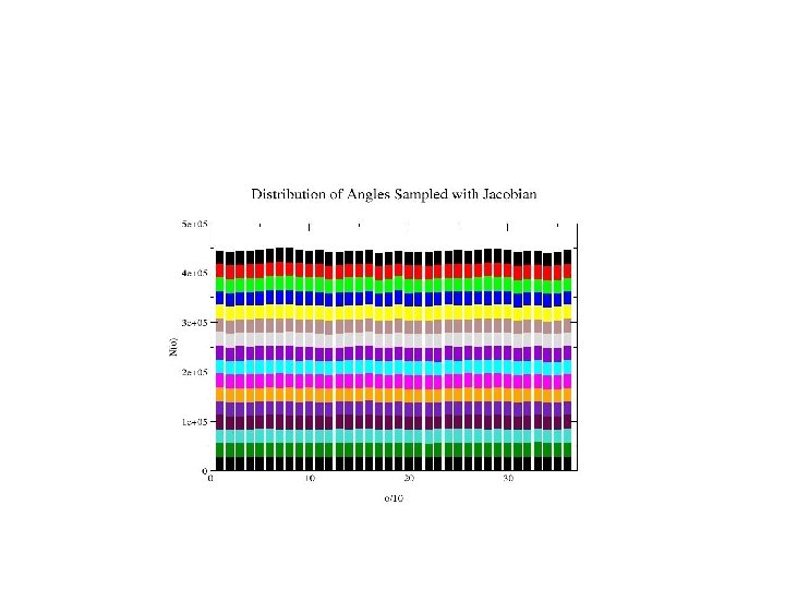
Methods of determining all zeros: (1) carry out resultant elimination; derive univariate polynomial of degree 16 solve using Sturm chains and deflation (2) carry out resultant elimination but convert matrix polynomial to a generalized eigenproblem of size 24 (3) work directly with trigonometric version; use geometry to define feasible intervals and exhaustively search. It is important to allow flexibility in some degrees of freedom

Loop Closure Algorithm 1. Polynomial coefficients are determined in terms of the geometric parameters on the right. 2. u 3 = tan( 3/2) is obtained by solving the polynomial equation. 3, 1, and 2 follow. 3. Positions of the all atoms are determined by transforming to the original frame. 1 2 3

General Chain Loop Closure

7 -Angle Loop Closure

Longer Loop Closure in Combination with an Existing Loop Construction Method Jacobson, et al, Proteins, 2004. Canutescu and Dunbrack, Protein Science, 12, 963 (2003).

Application to loop sampling Analytical closure of the two arms of a loop in the middle Comparison: 10 residue loop sampling (Matt Jacobson) No. of loops Numerical closure Analytical closure generated (best RMSD) 151 (1. 61) 40, 000 (1. 23) accepted (best RMSD) 1 (6. 75) 1, 374 (1. 58)

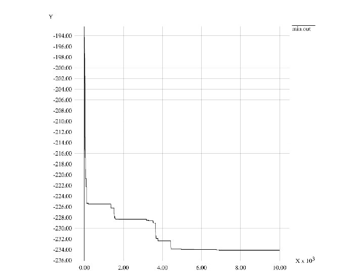
The continuous move used in Monte Carlo energy minimization

The continuous move: given a state assume D 2 b, D 4 a fixed, but D 3 variable tau 2 sigma 4 determined by D 3 (1) tau 1 sigma 2, tau 4 sigma 5 trivial (2) alpha 1, alpha 5 variable but depend only on vertices as do lengths (lengths 1 -2, 1 -5, 4 -5 are fixed) Given these sigma 1 tau 1, sigma 5 tau 5 known (sigma 1 tau 5 given) (3) Dihedral (2 -1 -5 -4) fixes remainder: alpha 2, alpha 4 determined (sigma 2 tau 2, sigma 4 tau 4 known)

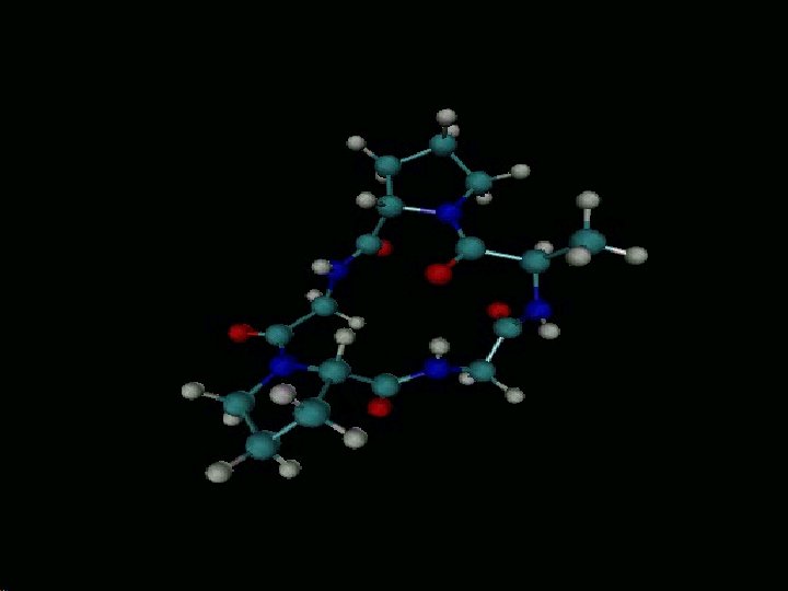
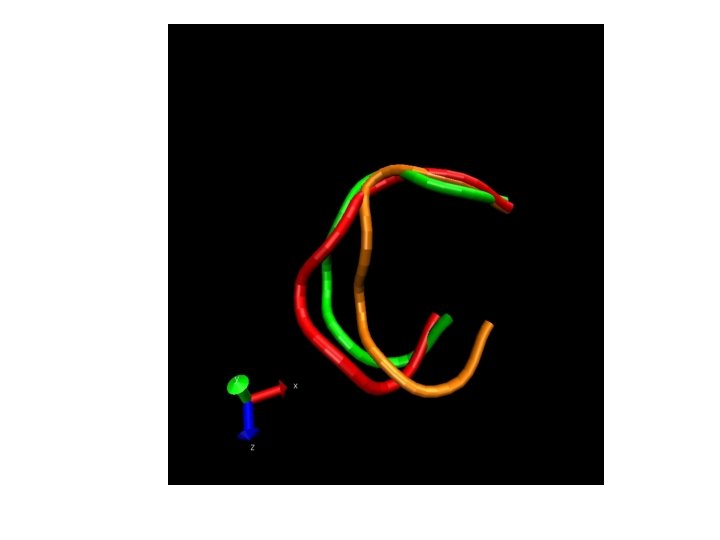
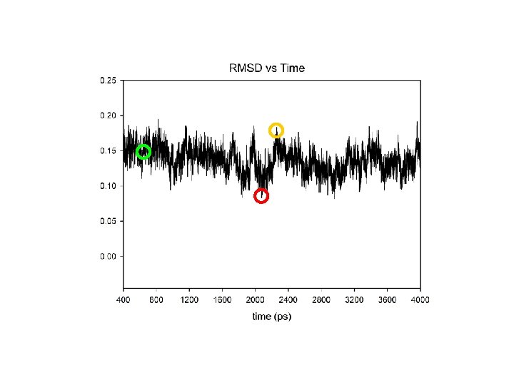
Refinement of 8 residue loop (84 -91) of turkey egg white lysozyme Native structure (red) and initial structure (blue) Baysal, C. and Meirovitch, H. , J. Phys. Chem. A, 1997, 101, 2185

3 peptide units are placed at the vertices of a triangle with random orientations, and they are connected by exact loop closure. The max and min values of the 3 -pep bridge set the limits for the sides of the triangle. Designing a 9 -peptide ring

In designing a 9 -peptide ring, the known parameters of 2 -pep bridges (and those of the S 2 bridge, if present) are incorporated in the choice of the foundation triangle, with vertices A, B, C (3 DOF) C B A

C B A peptide virtual bond (3 dof for placement)x 3=9 2 -pep virtual bond (at most 8 solutions) design triangle sides (3 dof )

8 -2 -4 4 -2 -4 Cyclic 9 -peptide backbone design 4 -6 -2 4 -2 -2 Numbers denote alternative loop closure solutions at each side of the brace triangle

Disulfide Loop Closure • Start at of the “last” Cysteine residue • The dihedral angle is a free variable: vary continuously to get all possible conformations. • Fix the bonds: and • Note that a move rooted at the “first” Cysteine must not fix but rather

Disulfide Bridge Loop Closure

pep virtual bond 3 -pep bridge design triangle C 9 -pep ring cysteine bridge 1 2 Modeling R. Larson’s 9 -peptide A Designing a 9 -peptide ring B 3

• Rotation of about the axis by angle (circle ) • Compensating rotation about the axis for the first peptide unit, by angle • This sets up the problem for the remaining peptide units as a dipeptide loop closure

PEP 25: CLLRMKSAC