Analysis of Power In SAS March 11 2013

Analysis of Power In SAS March 11, 2013 - Mariya Cheryomina

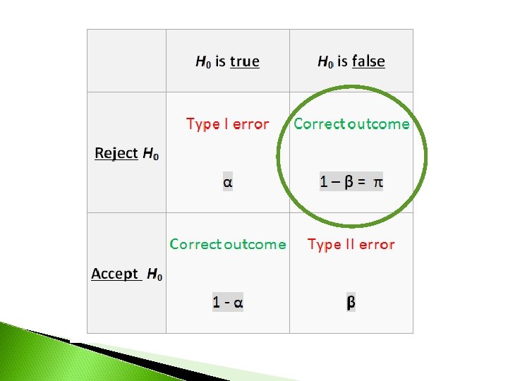
Power � power (π) + β = 1 � β = (1 - π) = probability of accepting false Ho (ie. reject true Ha) - probability of Type II error – false positive � Power (π) = (1 - β) = probability of detecting a difference when a difference does exist - probability of accepting true Ha (ie. reject false Ho) – how sensitive your test is to the existing difference between the compared samples

How do we know that power is large enough? � Generally, the minimal sufficient (acceptable) value of power is 0. 80 �π ≥ 0. 80

Analysis of power is performed: � 1) Before gathering data � To determine the minimal sample size needed to have desired power in statistical testing (to detect a particular effect size) � 2) After gathering data � To determine the magnitude of power that your statistical test will have given the sample parameters (n and s) and the magnitude of the effect that you want to detect

Power depends on: � Sample size (n) � Standard � Alpha deviation (s) level (α ) � Size of effect/difference that you want to detect � Type of statistical test performed

Analysis of power in SAS �One-sample �One-way t-test Anova

Analysis of power for one-sample t-test in SAS proc power; onesamplemeans mean = ____ ntotal = ____ stddev = ____ power = ____ ; run; (type of statistical test you want the power to be calculated for) (difference you are interested in detecting) (sample size) *One of the four variables must be left blank – this is what you want SAS to calculate

Example 1 You are asked to determine whether the use of a new soil type leads to a significantly different average height of young pine trees on plantation (compared to the historical/hypotherical mean height of 110 cm recorded with the old soil type). You want to conduct a one-sample t test with a 2 -sided α = 0. 05. You select 150 trees (n). You decide that the minimal difference in height worth addressing is 8 cm (effect size) α = 0. 05 s = 40 n = 150 “mean” = 8 (effect size) What will the power of your statistical test be? Ho: = 110 cm Ha: ≤ 102 cm OR ≥ 118 cm

Example 1 SAS text: proc power; onesamplemeans mean = 8 ntotal = 150 stddev = 40 power =. ; run; *Unless you indicate otherwise, SAS will automatically assume that α = 0. 05

SAS output: There is a there is a probability of 0. 68 that the t test will produce a significant result indicating a difference in mean tree height of at least 8 cm

Can choose different α level:

Try manipulating: � Sample size � Standard deviation

Visualizing power under different sample statistics You are interested in finding out how the changes in samples size (n), standard deviation (s) and minimal effect size of interest (“mean”) will effect the power of your one-sample t- test: proc power; onesamplemeans mean = 5 10 ntotal = 150 stddev = 30 50 power =. ; plot x=n min=100 max=200; run;

SAS output:

SAS output (continued): Effect size Increasing sample size does not infinitely increase power

One-way Anova Power Analysis Example 2: You want to compare the average diversity of Canada’s native bee species in four types of habitat: 1) Urban 2) Agricultural : Monoculture plantations (with pesticide use) 3) Agricultural : Organic farms (no pesticide use) 4) National parks � Ho: μ 1 = μ 2 = μ 3 = μ 4 Ha: one of μ is different

Example 2 (continued): What is the minimal number of sites of each habitat type that needs to be surveyed (ie. minimal sample size of each group) to detect whether a significant difference in bee species diversity exists between any of the four habitat types? (using a one-way Anova test with α = 0. 05) � The desired power of 0. 9. �

Example 2 (continued): *Analysis of power usually involves a number of simplifying assumptions Assumptions: Average number of bee species surveyed per site in Canada is ~35 species with a standard deviation of ~ 10 species Based on available research, you predict the following average bee species diversity for each habitat type: 1) Urban - 25 species 2) Monoculture plantations - 30 species 3) Organic farms– 40 species 4) National parks – 45 species *Assume that all groups have the same stdev (s) All numbers used in example were invented for the purpose of the exercise

Example 2 – SAS procedure: proc power ; onewayanova groupmeans = 25| 30 | 45 stddev = 10 alpha = 0. 05 npergroup =. power =. 9; run;

SAS output: SAS finds the group sample size that gives a power (actual power) closest to the power you desire (ie. to the nominal power)

Example 2 - Conclusion � You will need to survey at least 7 locations with each of the four habitat types (ie. 7 urban sites, etc. ) to detect the desired (significant) difference between the mean diversities of bee species found at each of the habitat types

What if the desired detectable effect of habitat type of bee diversity was reduced? Now you are trying to detect a smaller difference between sample means (at a significant level) Observe the new minimal sample size for each group

Power (↑) when: Sample size (↑) X approaches when n approaches N � Standard deviation (↓) Difference between samples is less likely to cur simply due to random sampling effects � (α ) (↑) Higher α leads to lower β which results in higher power (ie. the more willing you are to reject Ho, the less likely you are to accept false Ho, which leads to a higher probability of detecting a truly existing significant difference) � Minimal effect size (↑) (difference that you want to detect) A large difference between samples is less likely to occur due to random variability between samples than a small difference is �

Suggestion � When you are expecting a large effect size, but are not fully confident that the true effect is as large, use a larger sample size (ie. one that the analysis of power suggests for detecting a smaller effect )

Useful sources: Analysis of power for Anova (in SAS): http: //www. ats. ucla. edu/stat/sas/dae/fpower. htm � Analysis of power for one-sample and two-sample t-tests (in SAS): http: //support. sas. com/rnd/app/papers/power. pdf �