SAS and all other SAS Institute Inc product

SAS and all other SAS Institute Inc. product or service names are registered trademarks or trademarks of SAS Institute Inc. in the USA and other countries. ® indicates USA registration. Other brand product names are trademarks of their respective companies.

Forecasting: Something Old, Something New David A. Dickey William Neal Reynolds Distinguished Professor of Statistics, NC State University Dr. Dickey has been on the NCSU Statistics faculty since 1976. He is fellow of the American Statistical Association and was a founding faculty member of the NCSU Institute for Advanced Analytics. Dave is a SAS® Books by Users author and has been a contract instructor for SAS since 1981. He has used SAS since 1976, using it daily in graduate level teaching and consulting. No Twitter handle. SAS and all other SAS Institute Inc. product or service names are registered trademarks or trademarks of SAS Institute Inc. in the USA and other countries. ® indicates USA registration. Other brand product names are trademarks of their respective companies. #SASGF

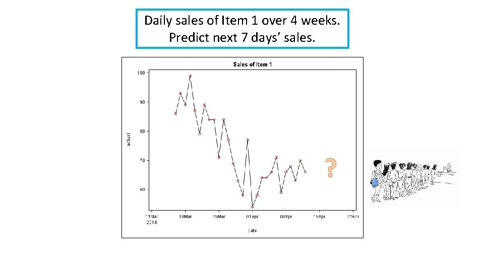
Daily sales of Item 1 over 4 weeks. Predict next 7 days’ sales. ?

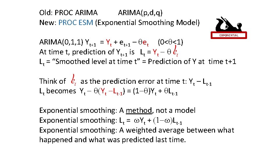
Old: PROC ARIMA(p, d, q) New: PROC ESM (Exponential Smoothing Model) EXPONENTIAL ARIMA(0, 1, 1) Yt+1 = Yt + et+1 – qet (0<q<1) At time t, prediction of Yt+1 is Lt = Yt - q Lt = “Smoothed level at time t” = Prediction of Y at time t+1 Think of as the prediction error at time t: Yt – Lt-1 Lt becomes Yt - q(Yt -Lt-1) = (1 -q)Yt + q. Lt-1 Exponential smoothing: A method, not a model Exponential smoothing: Lt = w. Yt + (1 -w)Lt-1 Exponential smoothing: A weighted average between what happened and what was predicted last time.

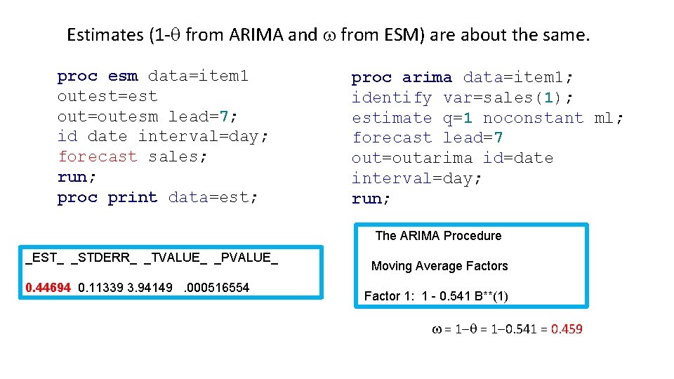
Estimates (1 -q from ARIMA and w from ESM) are about the same. proc esm data=item 1 outest=est out=outesm lead=7; id date interval=day; forecast sales; run; proc print data=est; proc arima data=item 1; identify var=sales(1); estimate q=1 noconstant ml; forecast lead=7 out=outarima id=date interval=day; run; The ARIMA Procedure _EST_ _STDERR_ _TVALUE_ _PVALUE_ 0. 44694 0. 11339 3. 94149. 000516554 Moving Average Factors Factor 1: 1 - 0. 541 B**(1) w = 1 -q = 1 -0. 541 = 0. 459

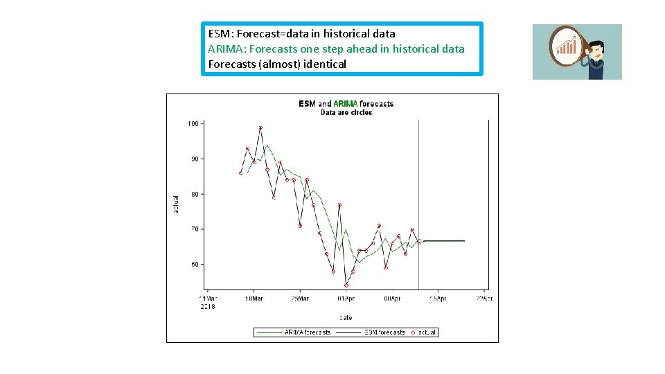
ESM: Forecast=data in historical data ARIMA: Forecasts one step ahead in historical data Forecasts (almost) identical

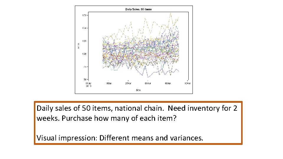
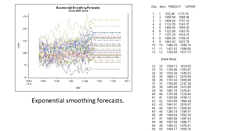
Daily sales of 50 items, national chain. Need inventory for 2 weeks. Purchase how many of each item? Visual impression: Different means and variances.

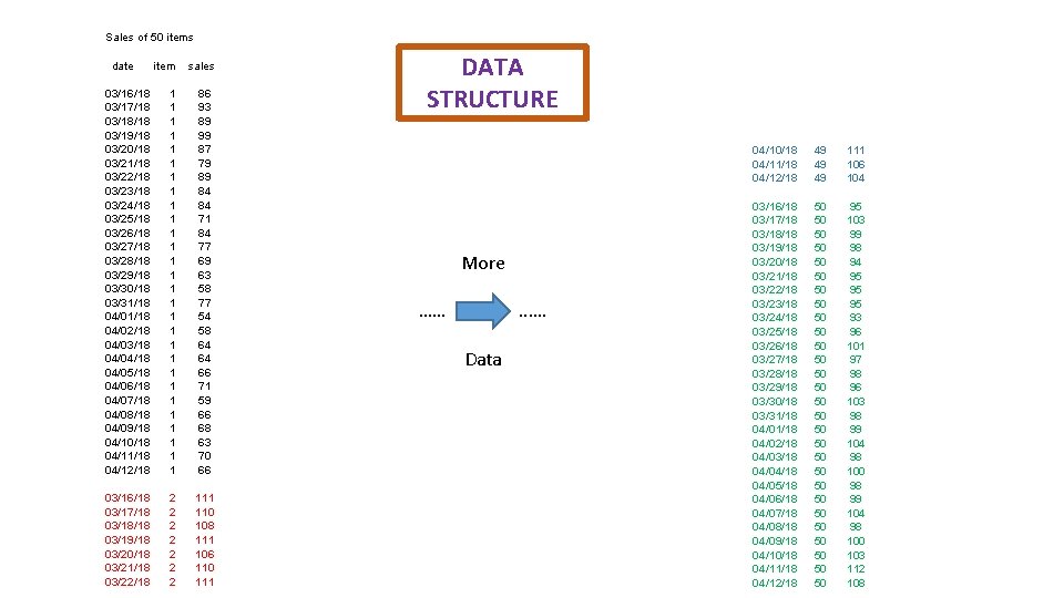
Sales of 50 items date item sales 03/16/18 03/17/18 03/18/18 03/19/18 03/20/18 03/21/18 03/22/18 03/23/18 03/24/18 03/25/18 03/26/18 03/27/18 03/28/18 03/29/18 03/30/18 03/31/18 04/02/18 04/03/18 04/04/18 04/05/18 04/06/18 04/07/18 04/08/18 04/09/18 04/10/18 04/11/18 04/12/18 1 1 1 1 1 1 1 86 93 89 99 87 79 89 84 84 71 84 77 69 63 58 77 54 58 64 64 66 71 59 66 68 63 70 66 03/16/18 03/17/18 03/18/18 03/19/18 03/20/18 03/21/18 03/22/18 2 2 2 2 111 110 108 111 106 110 111 DATA STRUCTURE More …… . . …. 04/10/18 04/11/18 04/12/18 49 49 49 111 106 104 03/16/18 03/17/18 03/18/18 03/19/18 03/20/18 03/21/18 03/22/18 03/23/18 03/24/18 03/25/18 03/26/18 03/27/18 03/28/18 03/29/18 03/30/18 03/31/18 04/02/18 04/03/18 04/04/18 04/05/18 04/06/18 04/07/18 04/08/18 04/09/18 04/10/18 04/11/18 04/12/18 50 50 50 50 50 50 50 95 103 99 98 94 95 95 95 93 96 101 97 98 96 103 98 99 104 98 100 103 112 108 Data

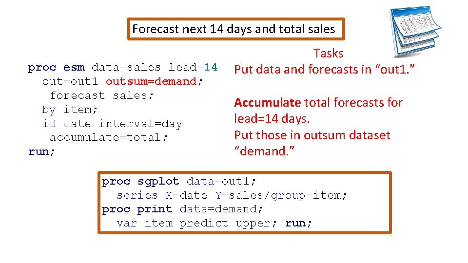
Forecast next 14 days and total sales proc esm data=sales lead=14 out=out 1 outsum=demand; forecast sales; by item; id date interval=day accumulate=total; run; Tasks Put data and forecasts in “out 1. ” Accumulate total forecasts for lead=14 days. Put those in outsum dataset “demand. ” proc sgplot data=out 1; series X=date Y=sales/group=item; proc print data=demand; var item predict upper; run;

Obs item 1 2 3 4 5 6 7 8 9 10 11 12 PREDICT UPPER 932. 48 1173. 74 1856. 98 1999. 36 1604. 64 1751. 10 1132. 05 1243. 37 1854. 95 1959. 20 1322. 08 1363. 76 1337. 25 1434. 15 1665. 49 1789. 10 1643. 92 1822. 79 1488. 38 1580. 74 1421. 42 1586. 60 1352. 65 1517. 73 (more lines) Exponential smoothing forecasts. 32 33 34 35 36 37 38 39 40 41 42 43 44 45 46 47 48 49 50 1534. 12 1336. 96 1516. 26 1886. 12 1787. 43 1760. 80 1405. 68 1987. 76 1187. 69 1320. 68 1833. 59 1841. 61 1467. 61 1265. 19 1494. 54 1805. 99 1587. 94 1456. 22 1494. 17 1616. 63 1353. 97 1545. 02 2079. 95 1859. 99 2157. 28 1472. 60 2376. 81 1218. 40 1536. 12 1896. 48 2016. 97 1609. 85 1394. 57 1562. 29 1897. 43 1886. 77 1476. 41 1605. 76

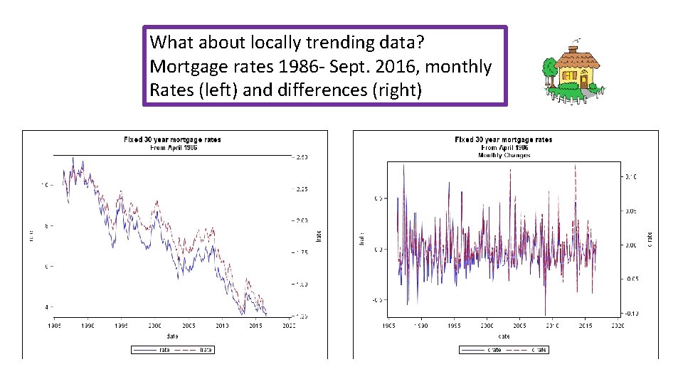
What about locally trending data? Mortgage rates 1986 - Sept. 2016, monthly Rates (left) and differences (right)

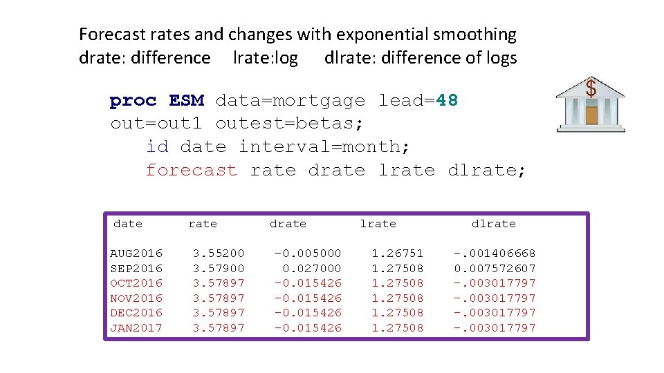
Forecast rates and changes with exponential smoothing drate: difference lrate: log dlrate: difference of logs proc ESM data=mortgage lead=48 out=out 1 outest=betas; id date interval=month; forecast rate drate lrate dlrate; date AUG 2016 SEP 2016 OCT 2016 NOV 2016 DEC 2016 JAN 2017 rate 3. 55200 3. 57900 3. 57897 drate -0. 005000 0. 027000 -0. 015426 lrate 1. 26751 1. 27508 dlrate -. 001406668 0. 007572607 -. 003017797

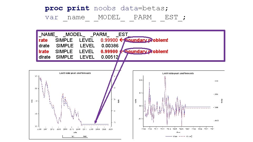
proc print noobs data=betas; var _name_ _MODEL_ _PARM_ _EST_; _NAME_ _MODEL_ _PARM_ _EST_ rate SIMPLE LEVEL 0. 99900 boundary problem! drate SIMPLE LEVEL 0. 00386 lrate SIMPLE LEVEL 0. 99900 boundary problem! dlrate SIMPLE LEVEL 0. 00512

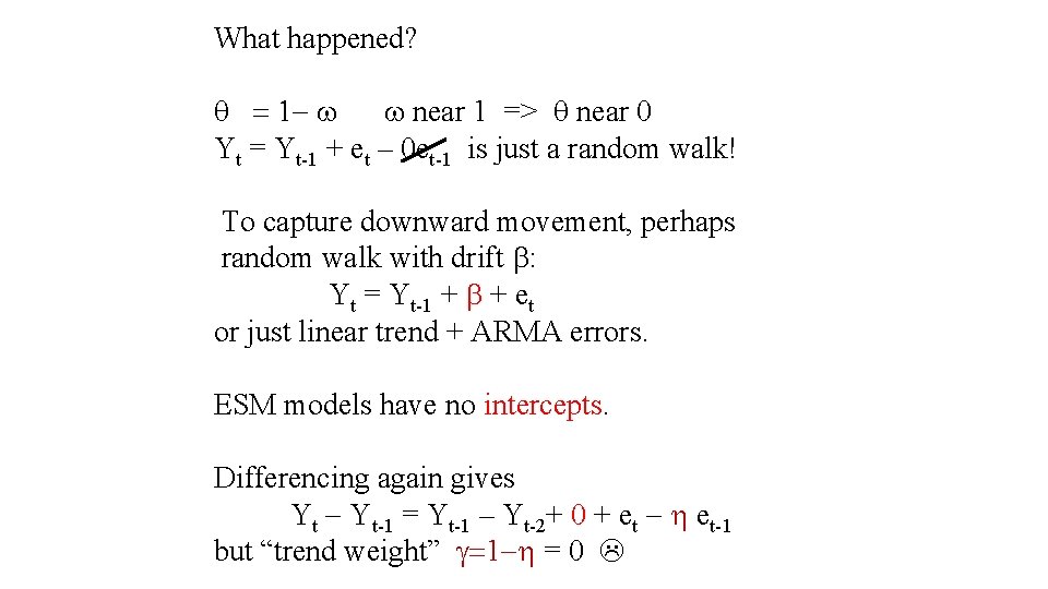
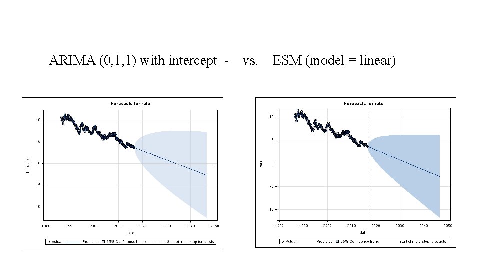
What happened? q = 1 - w w near 1 => q near 0 Yt = Yt-1 + et – 0 et-1 is just a random walk! To capture downward movement, perhaps random walk with drift b: Yt = Yt-1 + b + et or just linear trend + ARMA errors. ESM models have no intercepts. Differencing again gives Yt - Yt-1 = Yt-1 – Yt-2+ 0 + et - h et-1 but “trend weight” g=1 -h = 0

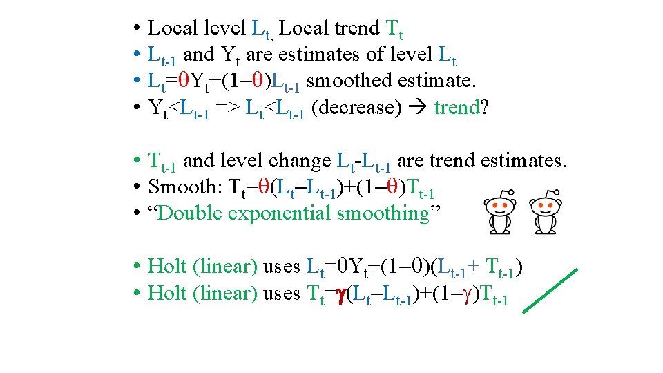
• • Local level Lt, Local trend Tt Lt-1 and Yt are estimates of level Lt Lt=q. Yt+(1 -q)Lt-1 smoothed estimate. Yt<Lt-1 => Lt<Lt-1 (decrease) trend? • Tt-1 and level change Lt-Lt-1 are trend estimates. • Smooth: Tt=q(Lt-Lt-1)+(1 -q)Tt-1 • “Double exponential smoothing” • Holt (linear) uses Lt=q. Yt+(1 -q)(Lt-1+ Tt-1) • Holt (linear) uses Tt=g(Lt-Lt-1)+(1 -g)Tt-1

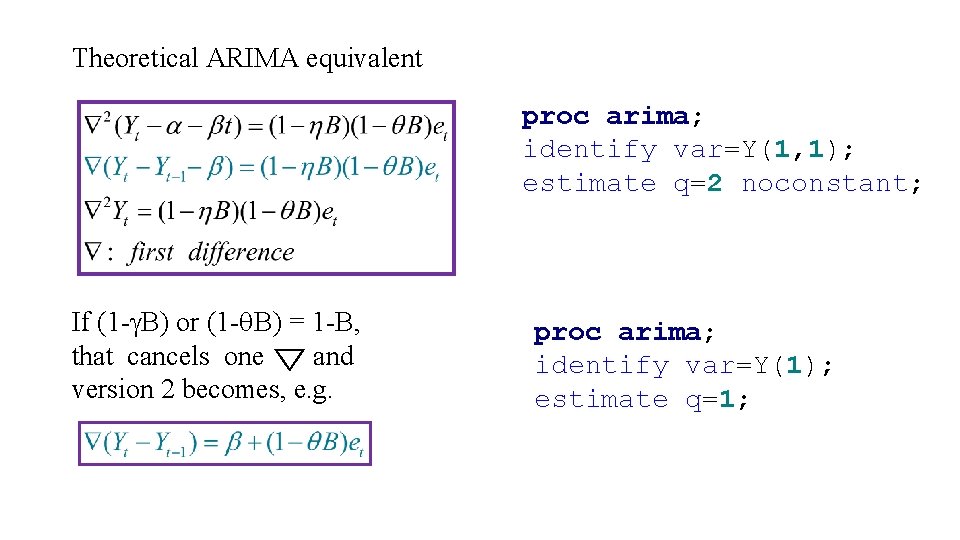
Theoretical ARIMA equivalent proc arima; identify var=Y(1, 1); estimate q=2 noconstant; If (1 -g. B) or (1 -q. B) = 1 -B, that cancels one and version 2 becomes, e. g. proc arima; identify var=Y(1); estimate q=1;

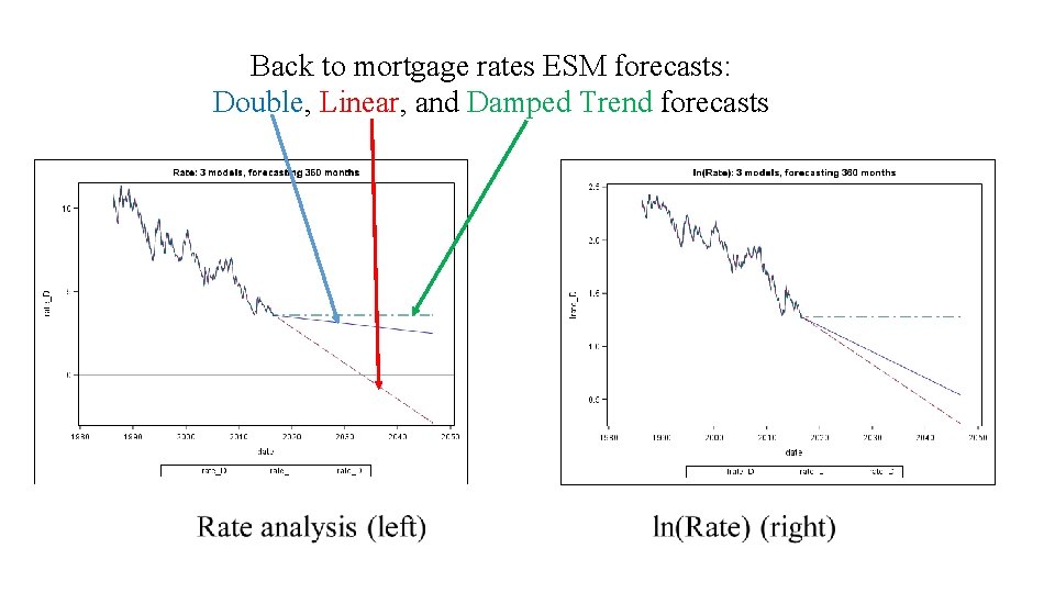
Back to mortgage rates ESM forecasts: Double, Linear, and Damped Trend forecasts

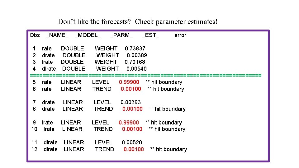
Don’t like the forecasts? Check parameter estimates! Obs _NAME_ _MODEL_ _PARM_ _EST_ error 1 rate DOUBLE WEIGHT 0. 73837 2 drate DOUBLE WEIGHT 0. 00389 3 lrate DOUBLE WEIGHT 0. 70168 4 dlrate DOUBLE WEIGHT 0. 00540 ==================================== 5 rate LINEAR LEVEL 0. 99900 ** hit boundary 6 rate LINEAR TREND 0. 00100 ** hit boundary 7 8 drate LINEAR LEVEL TREND 9 lrate 10 lrate LINEAR LEVEL TREND 11 12 dlrate 0. 00393 0. 00100 ** hit boundary 0. 99900 ** hit boundary 0. 00100 ** hit boundary 0. 00520 0. 00100 ** hit boundary

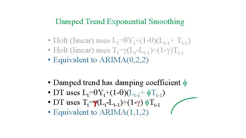
Damped Trend Exponential Smoothing • Holt (linear) uses Lt=q. Yt+(1 -q)(Lt-1+ Tt-1) • Holt (linear) uses Tt=g(Lt-Lt-1)+(1 -g)Tt-1 • Equivalent to ARIMA(0, 2, 2) • • Damped trend has damping coefficient f DT uses Lt=q. Yt+(1 -q)(Lt-1+ f. Tt-1) DT uses Tt=g(Lt-Lt-1)+(1 -g) f. Tt-1 Equivalent to ARIMA(1, 1, 2)

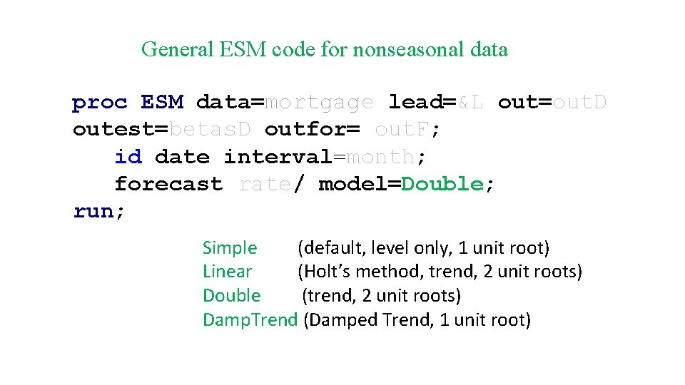
General ESM code for nonseasonal data proc ESM data=mortgage lead=&L out=out. D outest=betas. D outfor= out. F; id date interval=month; forecast rate/ model=Double; run; Simple (default, level only, 1 unit root) Linear (Holt’s method, trend, 2 unit roots) Double (trend, 2 unit roots) Damp. Trend (Damped Trend, 1 unit root)

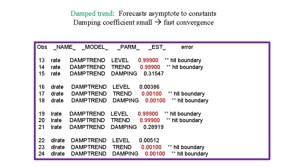
Damped trend: Forecasts asymptote to constants Damping coefficient small fast convergence Obs _NAME_ _MODEL_ _PARM_ _EST_ error 13 14 15 rate DAMPTREND LEVEL 0. 99900 ** hit boundary TREND 0. 99900 ** hit boundary DAMPING 0. 31547 16 17 18 drate DAMPTREND LEVEL 0. 00386 TREND 0. 00100 ** hit boundary DAMPING 0. 00100 ** hit boundary 19 20 21 lrate DAMPTREND LEVEL 0. 99900 ** hit boundary TREND 0. 99900 ** hit boundary DAMPING 0. 28919 22 23 24 dlrate DAMPTREND LEVEL 0. 00512 TREND 0. 00100 ** hit boundary DAMPING 0. 00100 ** hit boundary

ARIMA (0, 1, 1) with intercept - vs. ESM (model = linear)

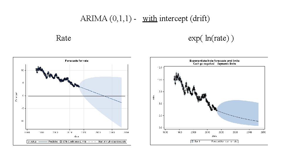
ARIMA (0, 1, 1) - with intercept (drift) Rate exp( ln(rate) )

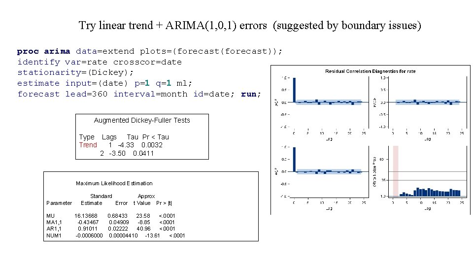
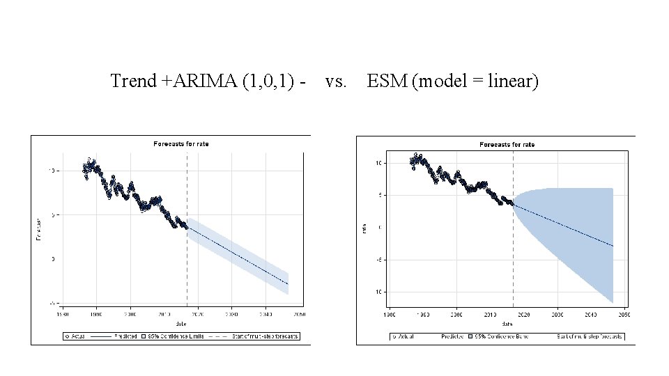
Try linear trend + ARIMA(1, 0, 1) errors (suggested by boundary issues) proc arima data=extend plots=(forecast)); identify var=rate crosscor=date stationarity=(Dickey); estimate input=(date) p=1 q=1 ml; forecast lead=360 interval=month id=date; run; Augmented Dickey-Fuller Tests Type Lags Tau Pr < Tau Trend 1 -4. 33 0. 0032 2 -3. 50 0. 0411 Maximum Likelihood Estimation Parameter MU MA 1, 1 AR 1, 1 NUM 1 Standard Estimate Error Approx t Value Pr > |t| 16. 13668 0. 68433 23. 58 <. 0001 -0. 43467 0. 04909 -8. 85 <. 0001 0. 91011 0. 02222 40. 96 <. 0001 -0. 0006000 0. 00004410 -13. 61 <. 0001

Trend +ARIMA (1, 0, 1) - vs. ESM (model = linear)

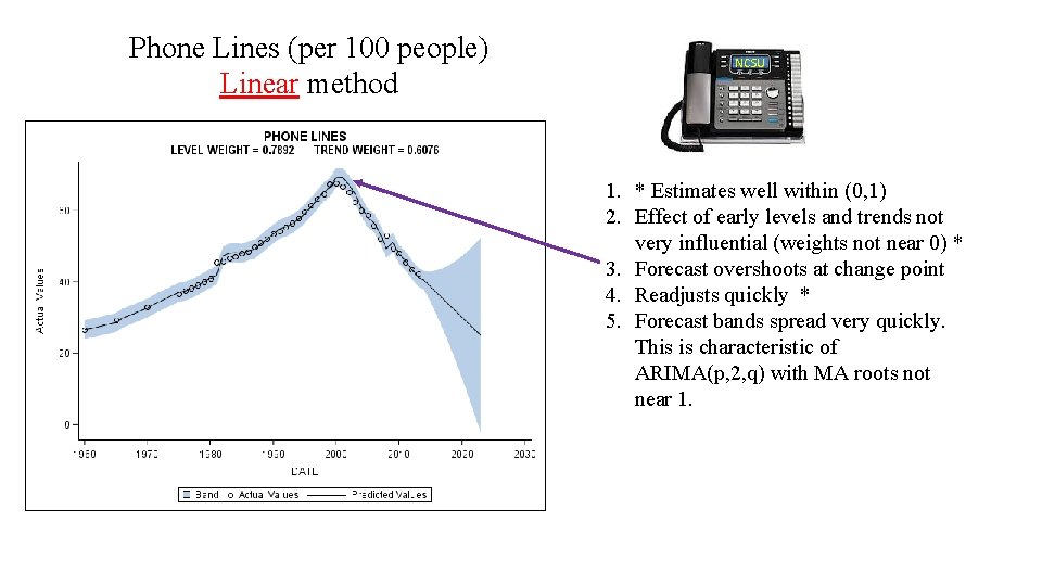
Phone Lines (per 100 people) Linear method NCSU 1. * Estimates well within (0, 1) 2. Effect of early levels and trends not very influential (weights not near 0) * 3. Forecast overshoots at change point 4. Readjusts quickly * 5. Forecast bands spread very quickly. This is characteristic of ARIMA(p, 2, q) with MA roots not near 1.

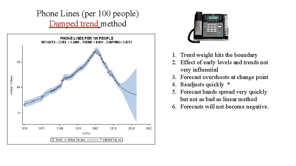
Phone Lines (per 100 people) Damped trend method NCSU 1. Trend weight hits the boundary 2. Effect of early levels and trends not very influential 3. Forecast overshoots at change point 4. Readjusts quickly * 5. Forecast bands spread very quickly but not as bad as linear method 6. Forecasts will not become negative.

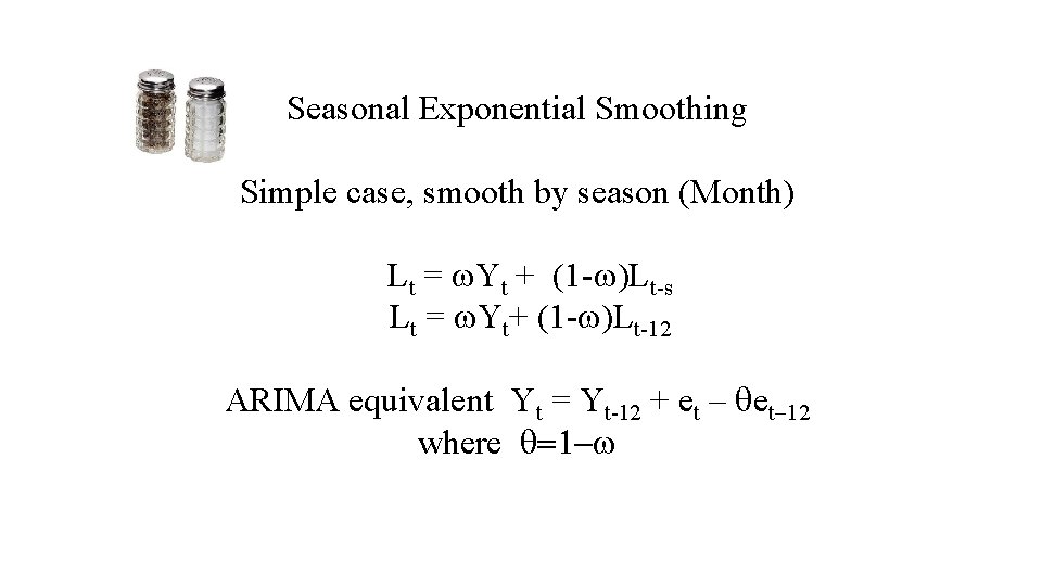
Seasonal Exponential Smoothing Simple case, smooth by season (Month) Lt = w. Yt + (1 -w)Lt-s Lt = w. Yt+ (1 -w)Lt-12 ARIMA equivalent Yt = Yt-12 + et – qet-12 where q=1 -w

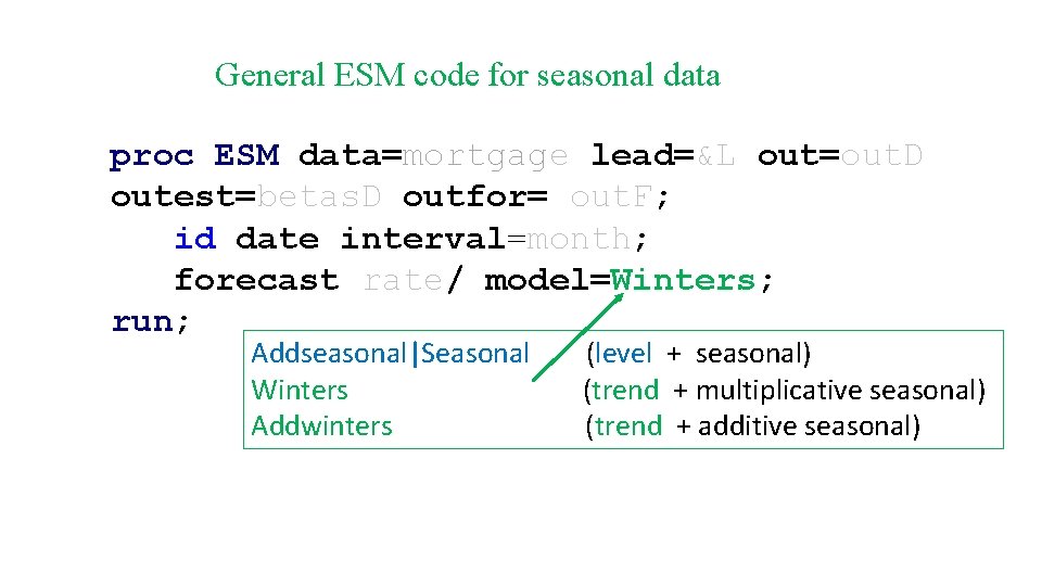
General ESM code for seasonal data proc ESM data=mortgage lead=&L out=out. D outest=betas. D outfor= out. F; id date interval=month; forecast rate/ model=Winters; run; Addseasonal|Seasonal (level + seasonal) Winters (trend + multiplicative seasonal) Addwinters (trend + additive seasonal)

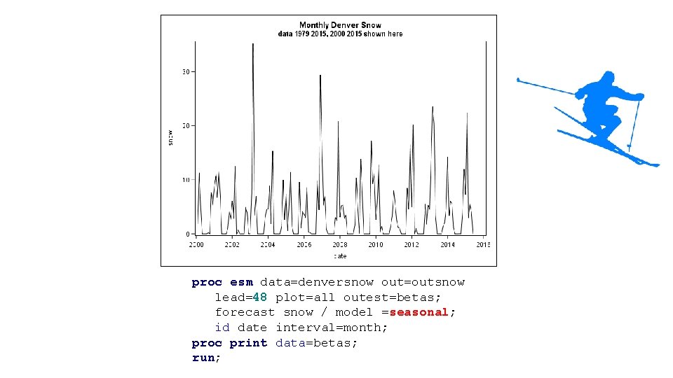
proc esm data=denversnow out=outsnow lead=48 plot=all outest=betas; forecast snow / model =seasonal; id date interval=month; proc print data=betas; run;

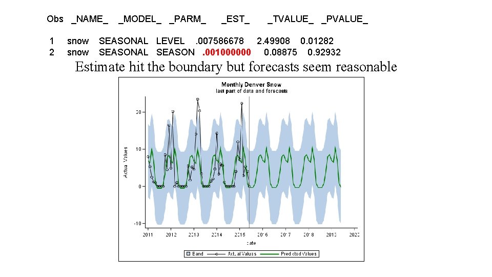
Obs _NAME_ 1 2 snow _MODEL_ _PARM_ _EST_ _TVALUE_ _PVALUE_ SEASONAL LEVEL. 007586678 2. 49908 0. 01282 SEASONAL SEASON. 001000000 0. 08875 0. 92932 Estimate hit the boundary but forecasts seem reasonable

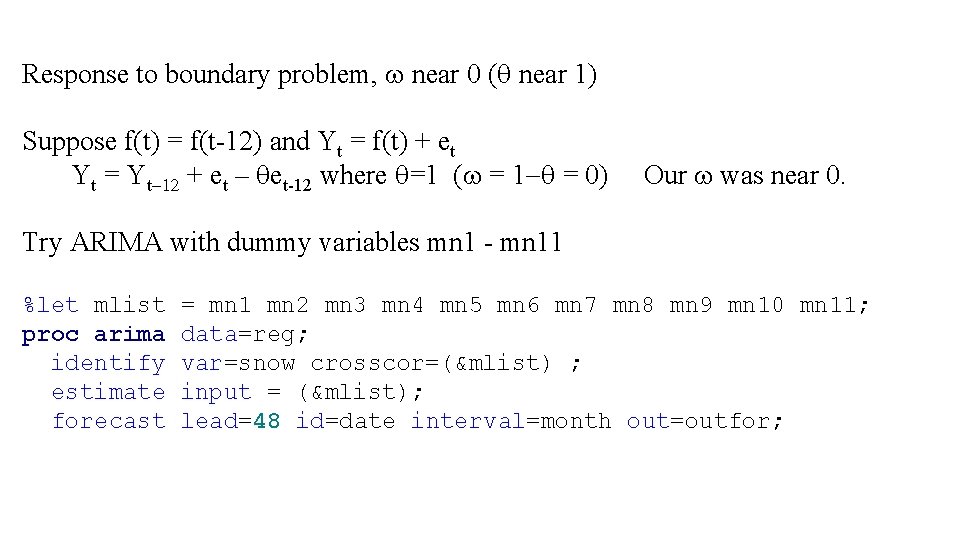
Response to boundary problem, w near 0 (q near 1) Suppose f(t) = f(t-12) and Yt = f(t) + et Yt = Yt-12 + et – qet-12 where q=1 (w = 1 -q = 0) Our w was near 0. Try ARIMA with dummy variables mn 1 - mn 11 %let mlist proc arima identify estimate forecast = mn 1 mn 2 mn 3 mn 4 mn 5 mn 6 mn 7 mn 8 mn 9 mn 10 mn 11; data=reg; var=snow crosscor=(&mlist) ; input = (&mlist); lead=48 id=date interval=month out=outfor;

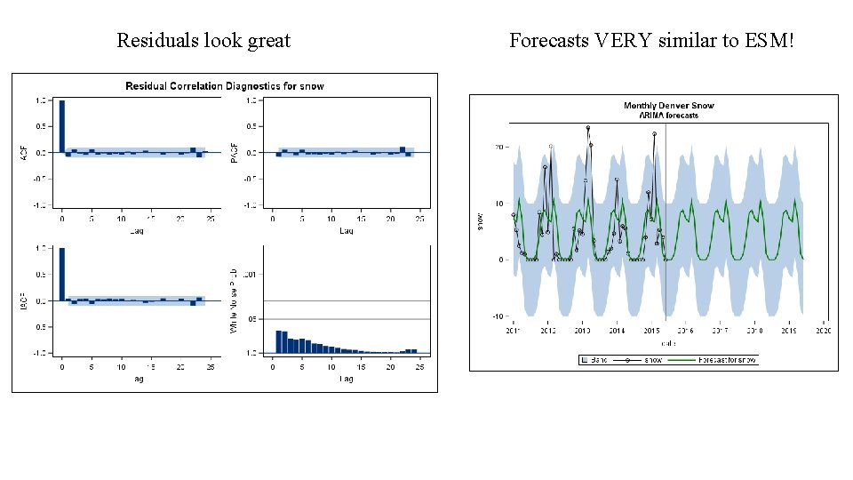
Residuals look great Forecasts VERY similar to ESM!

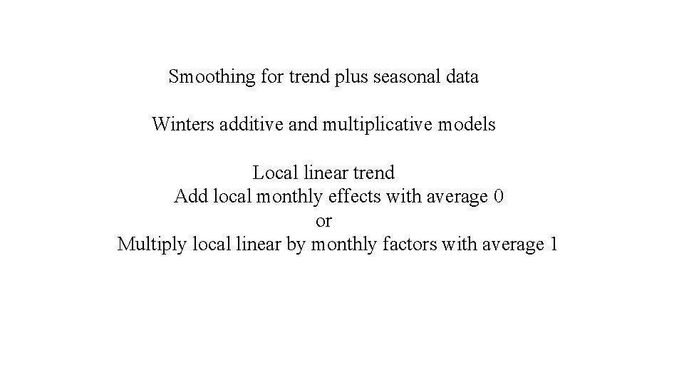
Smoothing for trend plus seasonal data Winters additive and multiplicative models Local linear trend Add local monthly effects with average 0 or Multiply local linear by monthly factors with average 1

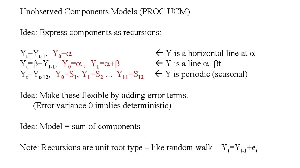
Unobserved Components Models (PROC UCM) Idea: Express components as recursions: Yt=Yt-1, Y 0=a Yt=b+Yt-1, Y 0=a , Y 1=a+b Yt=Yt-12, Y 0=S 1, Y 1=S 2 … Y 11=S 12 Y is a horizontal line at a Y is a line a+bt Y is periodic (seasonal) Idea: Make these flexible by adding error terms. (Error variance 0 implies deterministic) Idea: Model = sum of components Note: Recursions are unit root type – like random walk Yt=Yt-1+et

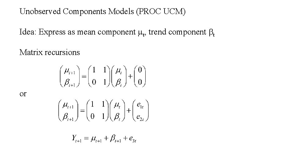
Unobserved Components Models (PROC UCM) Idea: Express as mean component mt, trend component bt Matrix recursions or

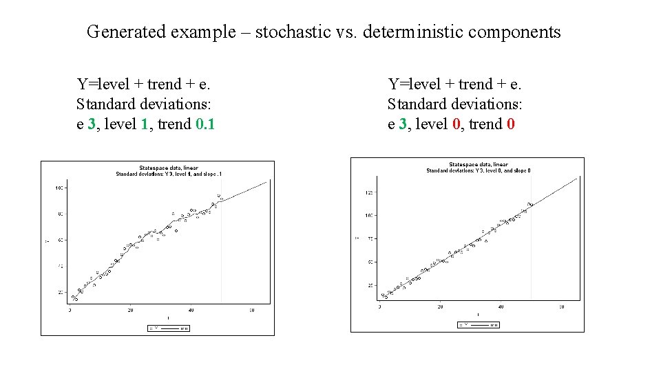
Generated example – stochastic vs. deterministic components Y=level + trend + e. Standard deviations: e 3, level 1, trend 0. 1 Y=level + trend + e. Standard deviations: e 3, level 0, trend 0

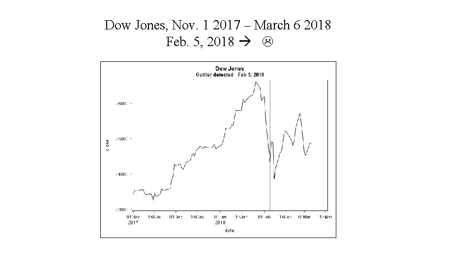
Dow Jones, Nov. 1 2017 – March 6 2018 Feb. 5, 2018

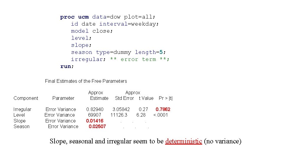
proc ucm data=dow plot=all; id date interval=weekday; model close; level; slope; season type=dummy length=5; irregular; ** error term **; run; Final Estimates of the Free Parameters Component Irregular Level Slope Season Parameter Error Variance Approx Estimate Approx Std Error t Value Pr > |t| 0. 82940 3. 05842 0. 27 0. 7862 69907 11126. 3 6. 28 <. 0001 0. 01416. . . 0. 02507. . . Slope, seasonal and irregular seem to be deterministic (no variance)

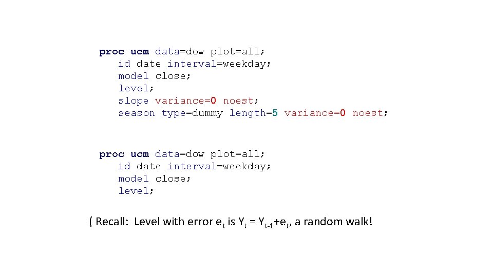
proc ucm data=dow plot=all; id date interval=weekday; model close; level; slope variance=0 noest; season type=dummy length=5 variance=0 noest; proc ucm data=dow plot=all; id date interval=weekday; model close; level; ( Recall: Level with error et is Yt = Yt-1+et, a random walk!

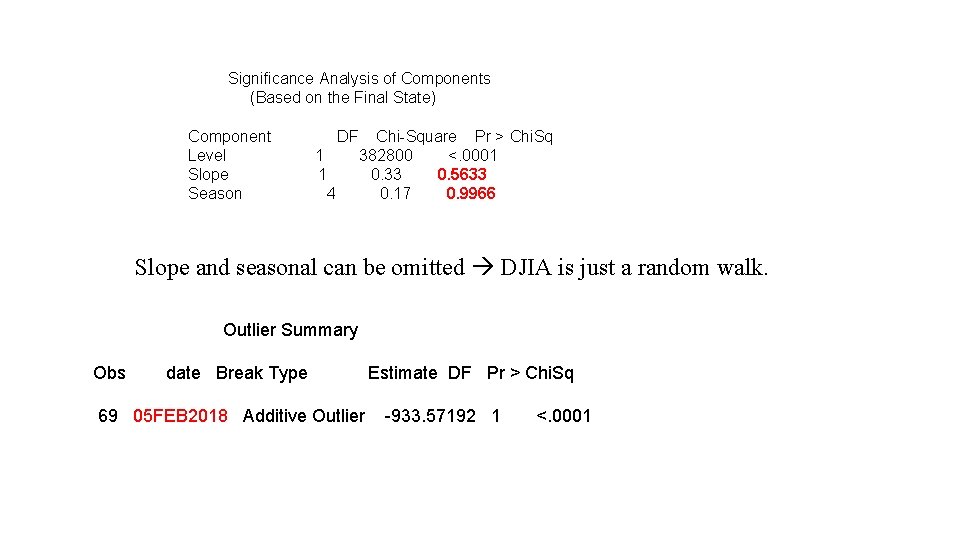
Significance Analysis of Components (Based on the Final State) Component Level Slope Season DF 1 1 4 Chi-Square Pr > Chi. Sq 382800 <. 0001 0. 33 0. 5633 0. 17 0. 9966 Slope and seasonal can be omitted DJIA is just a random walk. Outlier Summary Obs date Break Type 69 05 FEB 2018 Additive Outlier Estimate DF Pr > Chi. Sq -933. 57192 1 <. 0001

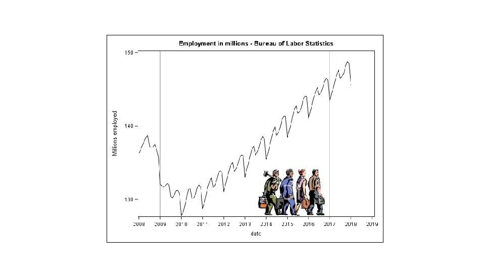
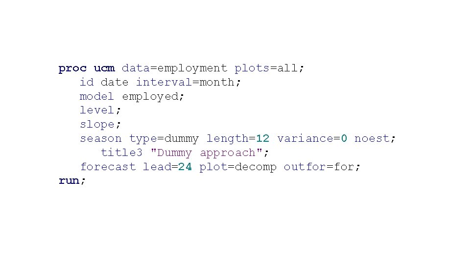
proc ucm data=employment plots=all; id date interval=month; model employed; level; slope; season type=dummy length=12 variance=0 noest; title 3 "Dummy approach"; forecast lead=24 plot=decomp outfor=for; run;

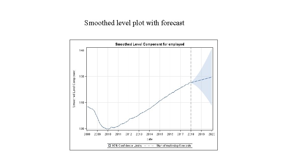
Smoothed level plot with forecast

Your Feedback Counts! Don't forget to complete the session survey in your conference mobile app. 1. Go to the Agenda icon in the conference app. 2. Find this session title and select it. 3. On the Sessions page, scroll down to Surveys and select the name of the survey. 4. Complete the survey and click Finish. #SASGF

SAS and all other SAS Institute Inc. product or service names are registered trademarks or trademarks of SAS Institute Inc. in the USA and other countries. ® indicates USA registration. Other brand product names are trademarks of their respective companies.

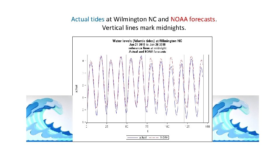
Actual tides at Wilmington NC and NOAA forecasts. Vertical lines mark midnights.

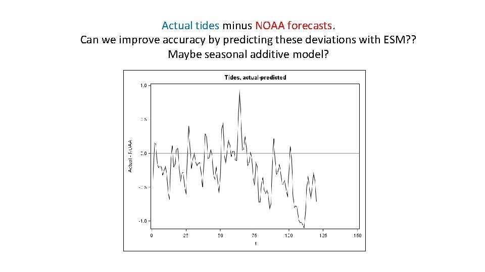
Actual tides minus NOAA forecasts. Can we improve accuracy by predicting these deviations with ESM? ? Maybe seasonal additive model?

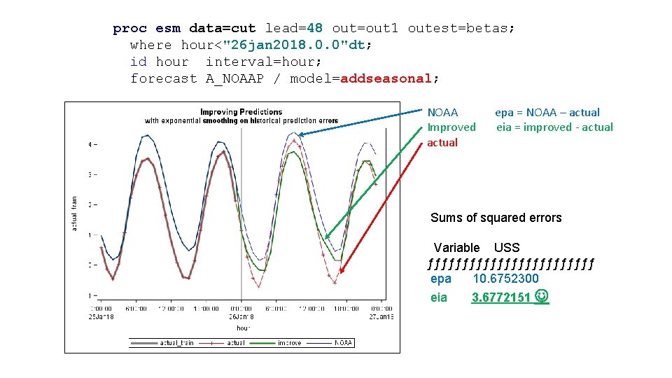
proc esm data=cut lead=48 out=out 1 outest=betas; where hour<"26 jan 2018. 0. 0"dt; id hour interval=hour; forecast A_NOAAP / model=addseasonal; NOAA epa = NOAA – actual Improved eia = improved - actual Sums of squared errors Variable USS ƒƒƒƒƒƒƒƒƒƒƒƒ epa 10. 6752300 eia 3. 6772151