Alternative lot sizing schemes Anadolu University Industrial Engineering

Alternative lot sizing schemes Anadolu University Industrial Engineering Department Source: Nahmias, S. , Production And Operations Analysis, Mc. Graw-Hill /Irwin, Fifth Edition, 2005, ISBN: 0073018651

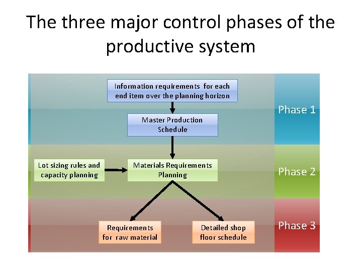
The three major control phases of the productive system Information requirements for each end item over the planning horizon Master Production Schedule Lot sizing rules and capacity planning Materials Requirements Planning Requirements for raw material Detailed shop floor schedule Phase 1 Phase 2 Phase 3

The explosion calculus • Explosion calculus is as term that refers to the set of rules by which gross requirements at one level of product structure are translated into a production schedule at that level and requirements at lower level. End item level Parent level (level 1) Child level (level 2) End item A(2) 1 week C(1) 2 weeks B(1) 2 weeks D(2) 1 week C(2) 2 weeks E(3) 2 weeks

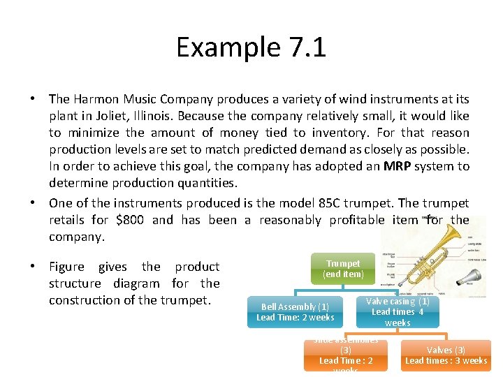
Example 7. 1 • The Harmon Music Company produces a variety of wind instruments at its plant in Joliet, Illinois. Because the company relatively small, it would like to minimize the amount of money tied to inventory. For that reason production levels are set to match predicted demand as closely as possible. In order to achieve this goal, the company has adopted an MRP system to determine production quantities. • One of the instruments produced is the model 85 C trumpet. The trumpet retails for $800 and has been a reasonably profitable item for the company. • Figure gives the product structure diagram for the construction of the trumpet. Trumpet (end item) Bell Assembly (1) Lead Time: 2 weeks Valve casing (1) Lead times 4 weeks Slide assemblies (3) Lead Time : 2 weeks Valves (3) Lead times : 3 weeks

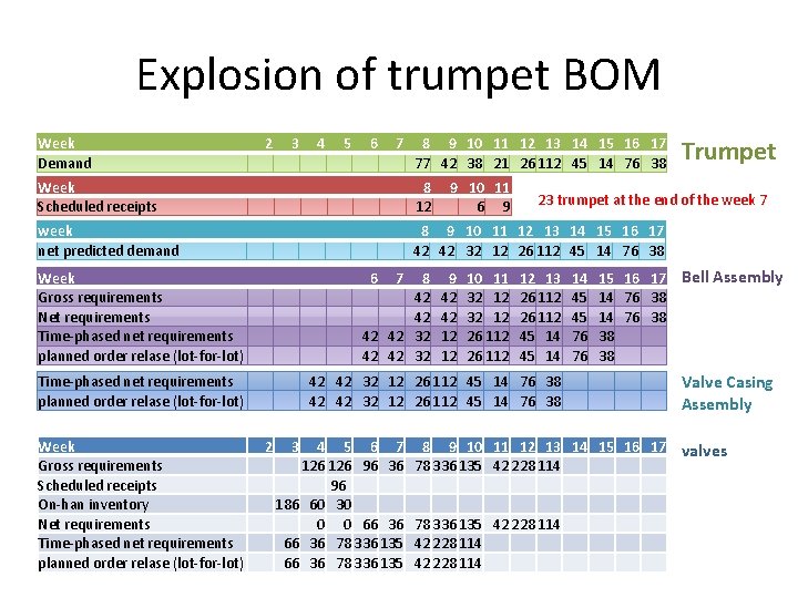
Explosion of trumpet BOM Week Demand 2 3 4 5 6 7 8 9 10 11 12 13 14 15 16 17 77 42 38 21 26 112 45 14 76 38 Week Scheduled receipts 8 12 week net predicted demand 8 9 10 11 12 13 14 15 16 17 42 42 32 12 26 112 45 14 76 38 Week Gross requirements Net requirements Time-phased net requirements planned order relase (lot-for-lot) 6 8 42 42 32 Time-phased net requirements planned order relase (lot-for-lot) Week Gross requirements Scheduled receipts On-han inventory Net requirements Time-phased net requirements planned order relase (lot-for-lot) 7 9 10 11 6 9 9 42 42 12 12 10 11 32 12 26 112 23 trumpet at the end of the week 7 12 13 26 112 45 14 42 42 32 12 26 112 45 14 76 38 2 3 4 5 6 7 126 96 36 96 186 60 30 0 0 66 36 78 336 135 Trumpet 14 45 45 76 76 15 16 17 Bell Assembly 14 76 38 38 38 Valve Casing Assembly 8 9 10 11 12 13 14 15 16 17 valves 78 336 135 42 228 114

Alternative Lot-Sizing Schemes • • EOQ lot sizing The silver-meal heuristic Least Unit Cost Part Period Balancing

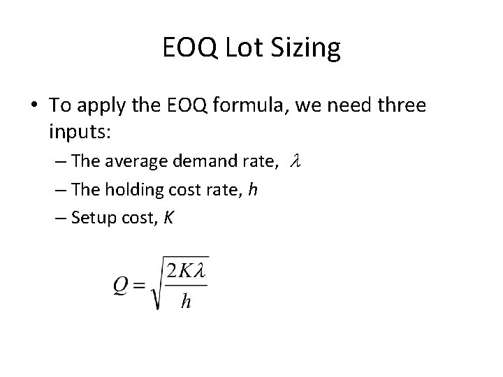
EOQ Lot Sizing • To apply the EOQ formula, we need three inputs: – The average demand rate, – The holding cost rate, h – Setup cost, K

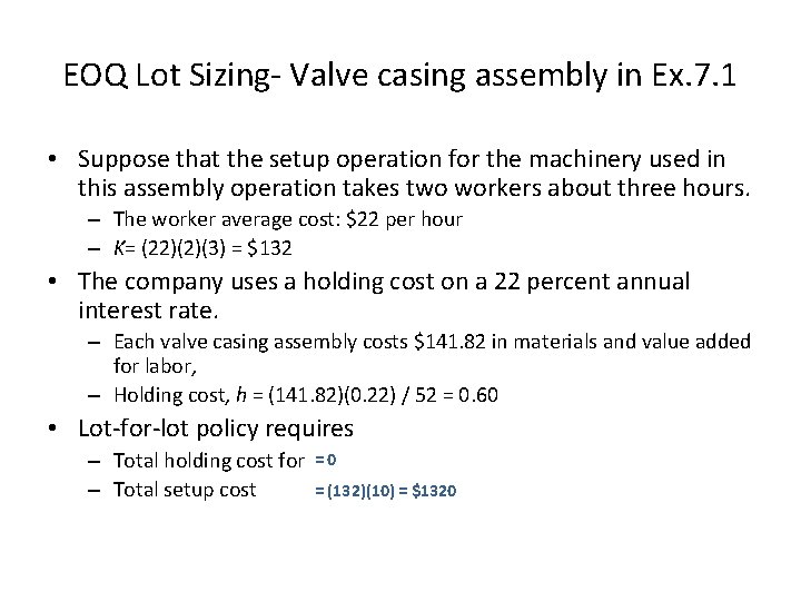
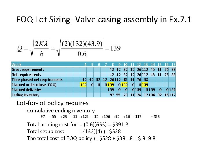
EOQ Lot Sizing- Valve casing assembly in Ex. 7. 1 • Suppose that the setup operation for the machinery used in this assembly operation takes two workers about three hours. – The worker average cost: $22 per hour – K= (22)(2)(3) = $132 • The company uses a holding cost on a 22 percent annual interest rate. – Each valve casing assembly costs $141. 82 in materials and value added for labor, – Holding cost, h = (141. 82)(0. 22) / 52 = 0. 60 • Lot-for-lot policy requires – Total holding cost for – Total setup cost =0 = (132)(10) = $1320

EOQ Lot Sizing- Valve casing assembly in Ex. 7. 1 Week Gross requirements Net requirements Time-phased net requirements Planned order relase (EOQ) Planned deliveries Ending inventory 4 5 6 7 8 9 10 42 42 32 12 26 112 45 139 0 0 0 139 139 0 0 97 55 23 11 12 13 14 12 26 112 45 14 76 38 0 0 139 11 124 12 106 15 16 17 14 76 38 0 0 139 92 16 117 Lot-for-lot policy requires Cumulative ending inventory 97 +55 +23 +11 +124 +12 +106 +92 +16 +117 = 653 Total holding cost for = (0. 6)(653) = $391. 8 Total setup cost = (132)(4) )= $528 The total cost of EOQ policy )= $528 + $391. 8 = $ 919. 8

The silver meal heuristic • The silver meal heuristic – named for Harlan Meal and Edward Silver – is a forward method that requires determining the average cost period as a function of the number of periods the current order is to span, – and stopping the computation when this function first increases. • C(T) as the average holding and setup cost period if the current orders spans the next T periods.

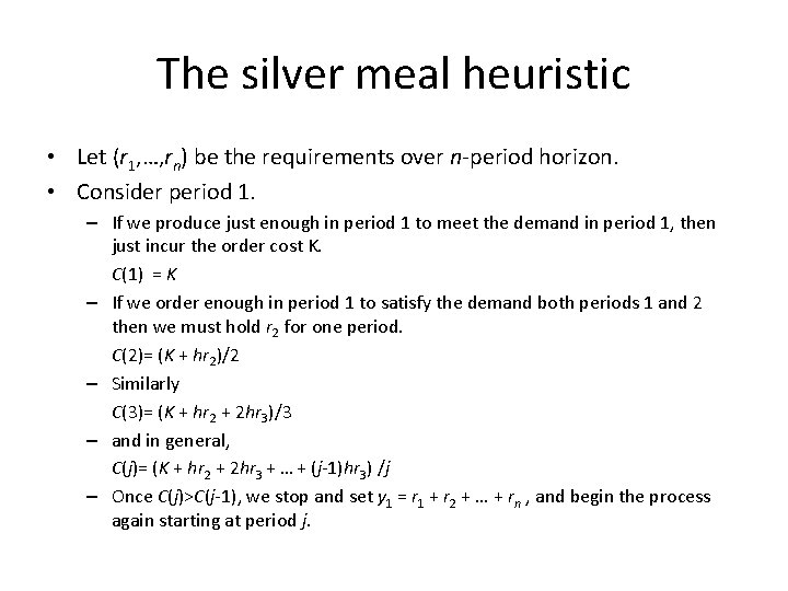
The silver meal heuristic • Let (r 1, …, rn) be the requirements over n-period horizon. • Consider period 1. – If we produce just enough in period 1 to meet the demand in period 1, then just incur the order cost K. C(1) = K – If we order enough in period 1 to satisfy the demand both periods 1 and 2 then we must hold r 2 for one period. C(2)= (K + hr 2)/2 – Similarly C(3)= (K + hr 2 + 2 hr 3)/3 – and in general, C(j)= (K + hr 2 + 2 hr 3 + … + (j-1)hr 3) /j – Once C(j)>C(j-1), we stop and set y 1 = r 1 + r 2 + … + rn , and begin the process again starting at period j.

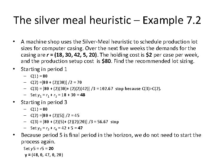
The silver meal heuristic – Example 7. 2 • A machine shop uses the Silver-Meal heuristic to schedule production lot sizes for computer casing. Over the next five weeks the demands for the casing are r = (18, 30, 42, 5, 20). The holding cost is $2 per case per week, and the production setup cost is $80. Find the recommended lot sizing. • Starting in period 1 – – C(1) = 80 C(2) =[80 + (2)(30)] /2 = 70 C(3) = [80 + (2)(30)+ (2)(2)(42)] /3 = 102. 67 stop because C(3)>C(2). Set y 1 = r 1 + r 2 = 18 + 30 = 48 • Starting in period 3 – – C(1) = 80 C(2) =[80 + (2)(5)] /2 = 45 C(3) = [80 + (2)(5)+ (2)(2)(20)] /3 = 56. 67 stop Set y 3 = r 3 + r 4 = 42 + 5 = 47 • Because period 5 is final period in the horizon, we do not need to start the process again. Set y 5 = r 5 = 20 y = (48, 0, 47, 0, 20)

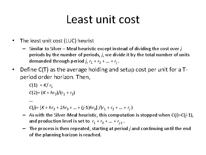
Least unit cost • The least unit cost (LUC) heurist – Similar to Silver – Meal heuristic except instead of dividing the cost over j periods by the number of periods, j, we divide it by the total number of units demanded through period j, r 1 + r 2 + … + rj. • Define C(T) as the average holding and setup cost per unit for a Tperiod order horizon. Then, C(1) = K/ r 1 C(2)= (K + hr 2)/(r 1 + r 2) … C(j)= [K + hr 2 + 2 hr 3 + … + (j-1)hr 3] /(r 1 + r 2 + … + rj ) – As with the Silver-Meal heuristic, this computation is stopped when C(j)>C(j-1), and production level is set to r 1 + r 2 + … + rj-1. – The process is then repeated, starting at period j and continuing until the end of the planning horizon is reached.

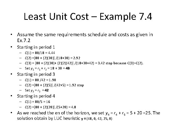
Least Unit Cost – Example 7. 4 • Assume the same requirements schedule and costs as given in Ex. 7. 2 • Starting in period 1 – – C(1) = 80/18 = 4. 44 C(2) =[80 + (2)(30)] /(18+30) = 2. 92 C(3) = [80 + (2)(30)+ (2)(2)(42)] /(18+30+42) = 3. 42 stop because C(3)>C(2). Set y 1 = r 1 + r 2 = 18 + 30 = 48 • Starting in period 3 – C(1) = 80 /42 = 1. 90 – C(2) =[80 + (2)(5)] /(42+5) = 1. 92 stop – Set y 3 = r 3 = 42 • Starting in period 4 – C(1) = 80/5 = 16 – C(2) =[80 + (2)(20)] /(5+20) = 4. 8 • As we reached the en of the horizon, we set y 4 = r 4 + r 5 = 5 + 20 =25. The solution obtain by LUC heuristic y = (48, 0, 42, 25, 0)

Part Period Balancing • Although Silver-Meal heuristic seems to give better results in a greater number of cases, part period balancing seems to be more popular in practice. • The method is set the order horizon equal to the number of periods that most closely matches the total holding cost with the setup cost over that period. • The order horizon that exactly equates holding and setup costs will rarely be an integer number of periods.

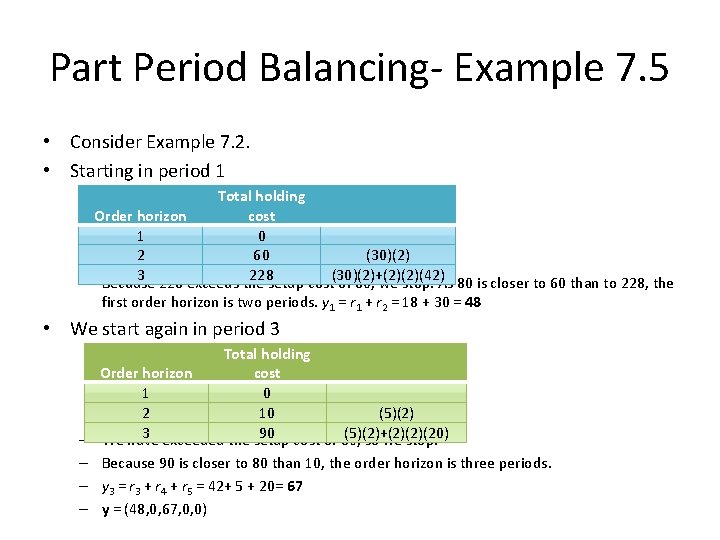
Part Period Balancing- Example 7. 5 • Consider Example 7. 2. • Starting in period 1 Total holding Order horizon cost 1 0 2 60 (30)(2) 3 228 exceeds the 228 setup cost(30)(2)+(2)(2)(42) – Because of 80, we stop. As 80 is closer to 60 than to 228, the first order horizon is two periods. y 1 = r 1 + r 2 = 18 + 30 = 48 • We start again in period 3 Total holding Order horizon cost 1 0 2 10 (5)(2) 3 exceeded the setup 90 cost of 80, (5)(2)+(2)(2)(20) – We have so we stop. – Because 90 is closer to 80 than 10, the order horizon is three periods. – y 3 = r 3 + r 4 + r 5 = 42+ 5 + 20= 67 – y = (48, 0, 67, 0, 0)

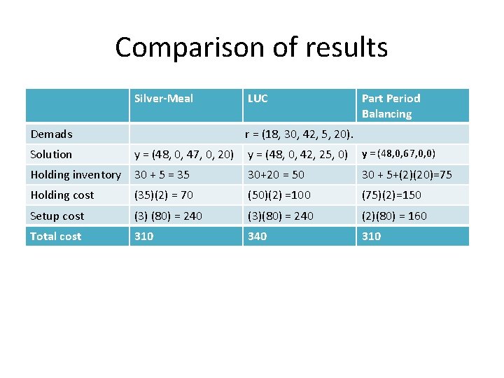
Comparison of results Silver-Meal Demads LUC Part Period Balancing r = (18, 30, 42, 5, 20). Solution y = (48, 0, 47, 0, 20) y = (48, 0, 42, 25, 0) y = (48, 0, 67, 0, 0) Holding inventory 30 + 5 = 35 30+20 = 50 30 + 5+(2)(20)=75 Holding cost (35)(2) = 70 (50)(2) =100 (75)(2)=150 Setup cost (3) (80) = 240 (3)(80) = 240 (2)(80) = 160 Total cost 310 340 310

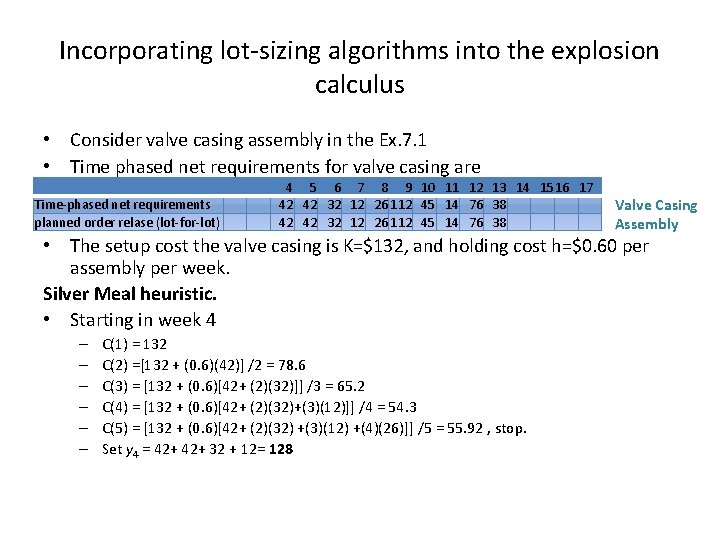
Incorporating lot-sizing algorithms into the explosion calculus • Consider valve casing assembly in the Ex. 7. 1 • Time phased net requirements for valve casing are Time-phased net requirements planned order relase (lot-for-lot) 4 5 6 7 8 9 10 11 12 13 14 15 16 17 42 42 32 12 26 112 45 14 76 38 Valve Casing Assembly • The setup cost the valve casing is K=$132, and holding cost h=$0. 60 per assembly per week. Silver Meal heuristic. • Starting in week 4 – – – C(1) = 132 C(2) =[132 + (0. 6)(42)] /2 = 78. 6 C(3) = [132 + (0. 6)[42+ (2)(32)]] /3 = 65. 2 C(4) = [132 + (0. 6)[42+ (2)(32)+(3)(12)]] /4 = 54. 3 C(5) = [132 + (0. 6)[42+ (2)(32) +(3)(12) +(4)(26)]] /5 = 55. 92 , stop. Set y 4 = 42+ 32 + 12= 128

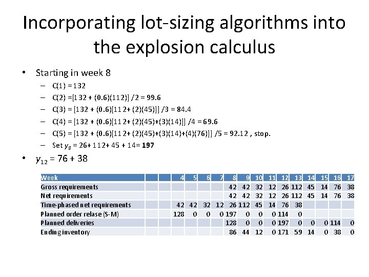
Incorporating lot-sizing algorithms into the explosion calculus • Starting in week 8 – – – C(1) = 132 C(2) =[132 + (0. 6)(112)] /2 = 99. 6 C(3) = [132 + (0. 6)[112+ (2)(45)]] /3 = 84. 4 C(4) = [132 + (0. 6)[112+ (2)(45)+(3)(14)]] /4 = 69. 6 C(5) = [132 + (0. 6)[112+ (2)(45)+(3)(14)+(4)(76)]] /5 = 92. 12 , stop. Set y 8 = 26+ 112+ 45 + 14= 197 • y 12 = 76 + 38 Week Gross requirements Net requirements Time-phased net requirements Planned order relase (S-M) Planned deliveries Ending inventory 4 5 6 7 8 42 42 32 12 26 128 0 0 0 197 128 86 9 42 42 112 0 0 44 10 32 32 45 0 0 12 11 12 12 14 0 0 0 12 26 26 76 114 197 171 13 112 38 0 0 59 14 15 16 17 45 14 76 38 0 14 0 114 0 38 0 0

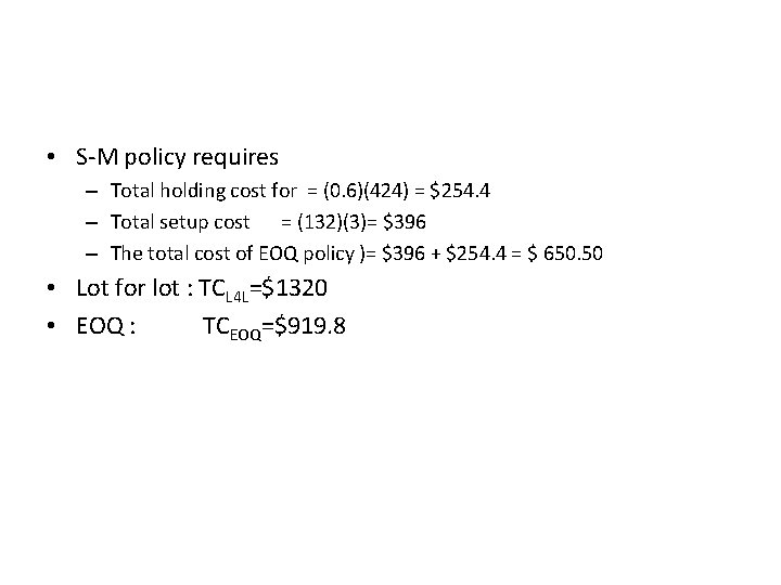
• S-M policy requires – Total holding cost for = (0. 6)(424) = $254. 4 – Total setup cost = (132)(3)= $396 – The total cost of EOQ policy )= $396 + $254. 4 = $ 650. 50 • Lot for lot : TCL 4 L=$1320 • EOQ : TCEOQ=$919. 8

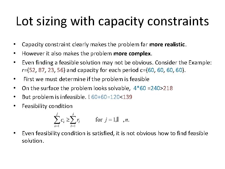
Lot sizing with capacity constraints • Capacity constraint clearly makes the problem far more realistic. • However it also makes the problem more complex. • Even finding a feasible solution may not be obvious. Consider the Example: r=(52, 87, 23, 56) and capacity for each period c=(60, 60, 60). • First we must determine if the problem is feasible • On the surface the problem looks solvable, 4*60 =240>218 • But problem is infeasible. ! 60+60=120<139 • Feasibility condition • Even feasibility condition is satisfied, it is not obvious how to find feasible solution.

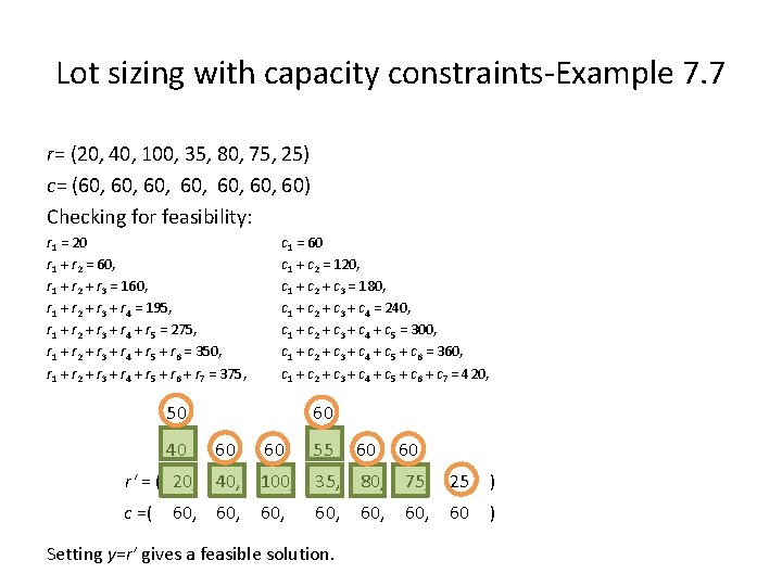
Lot sizing with capacity constraints-Example 7. 7 r= (20, 40, 100, 35, 80, 75, 25) c= (60, 60, 60, 60) Checking for feasibility: r 1 = 20 r 1 + r 2 = 60, r 1 + r 2 + r 3 = 160, r 1 + r 2 + r 3 + r 4 = 195, r 1 + r 2 + r 3 + r 4 + r 5 = 275, r 1 + r 2 + r 3 + r 4 + r 5 + r 6 = 350, r 1 + r 2 + r 3 + r 4 + r 5 + r 6 + r 7 = 375, c 1 = 60 c 1 + c 2 = 120, c 1 + c 2 + c 3 = 180, c 1 + c 2 + c 3 + c 4 = 240, c 1 + c 2 + c 3 + c 4 + c 5 = 300, c 1 + c 2 + c 3 + c 4 + c 5 + c 6 = 360, c 1 + c 2 + c 3 + c 4 + c 5 + c 6 + c 7 = 420, 50 40 60 60 60 55 60 r‘ = ( 20, 40, 100, 35, 80, 75, 25 ) c =( 60, 60 ) 60, Setting y=r’ gives a feasible solution. 60

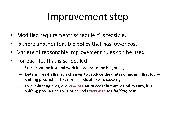
Improvement step • • Modified requirements schedule r’ is feasible. Is there another feasible policy that has lower cost. Variety of reasonable improvement rules can be used For each lot that is scheduled – Start from the last and work backward to the beginning – Determine whether it is cheaper to produce the units composing that lot by shifting production to prior periods of excess capacity – By eliminating a lot, one reduces setup const in that period to zero, but shifting production to prior periods increases the holding cost.

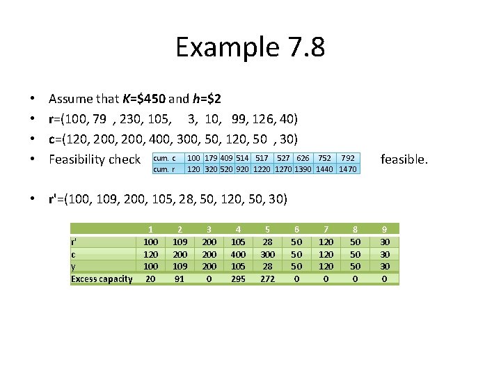
Example 7. 8 • • Assume that K=$450 and h=$2 r=(100, 79 , 230, 105, 3, 10, 99, 126, 40) c=(120, 200, 400, 300, 50, 120, 50 , 30) Feasibility check cum. c 100 179 409 514 517 527 626 cum. r 752 792 120 320 520 920 1270 1390 1440 1470 feasible. • r'=(100, 109, 200, 105, 28, 50, 120, 50, 30) r' c y Excess capacity 1 100 120 100 20 2 109 200 109 91 3 200 200 0 4 105 400 105 295 5 28 300 28 272 6 50 50 50 0 7 120 120 0 8 50 50 50 0 9 30 30 30 0

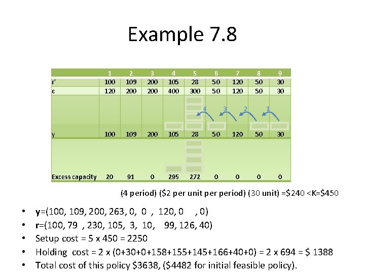
Example 7. 8 r' c y Excess capacity 1 100 120 100 20 2 109 200 109 91 3 200 4 105 400 263 105 0 137 295 5 6 7 28 50 120 300 50 120 0 158 4 3 2 108 58 0 28 50 120 300 142 192 242 272 0 0 8 50 50 9 30 30 1 0 50 0 30 0 0 (4 period) ($2 per unit period) (30 unit) =$240 <K=$450 • • • y=(100, 109, 200, 263, 0, 0 , 120, 0 , 0) r=(100, 79 , 230, 105, 3, 10, 99, 126, 40) Setup cost = 5 x 450 = 2250 Holding cost = 2 x (0+30+0+158+155+145+166+40+0) = 2 x 694 = $ 1388 Total cost of this policy $3638, ($4482 for initial feasible policy).

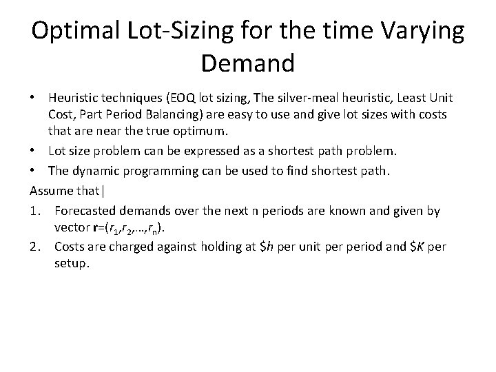
Optimal Lot-Sizing for the time Varying Demand • Heuristic techniques (EOQ lot sizing, The silver-meal heuristic, Least Unit Cost, Part Period Balancing) are easy to use and give lot sizes with costs that are near the true optimum. • Lot size problem can be expressed as a shortest path problem. • The dynamic programming can be used to find shortest path. Assume that| 1. Forecasted demands over the next n periods are known and given by vector r=(r 1, r 2, …, rn). 2. Costs are charged against holding at $h per unit period and $K per setup.

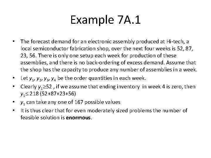
Example 7 A. 1 • The forecast demand for an electronic assembly produced at Hi-tech, a local semiconductor fabrication shop, over the next four weeks is 52, 87, 23, 56. There is only one setup each week for production of these assemblies, and there is no back-ordering of excess demand. Assume that the shop has the capacity to produce any number of assemblies in a week. • Let y 1, y 2, y 3, y 4 be the order quantities in each week. • Clearly y 1 52 , if we assume that ending inventory in week 4 is zero, then y 1 218 (52+87+23+56) • y 1 can take any one of 167 possible values • It is thus clear that for even moderately sized problems the number of feasible solution is enormous.

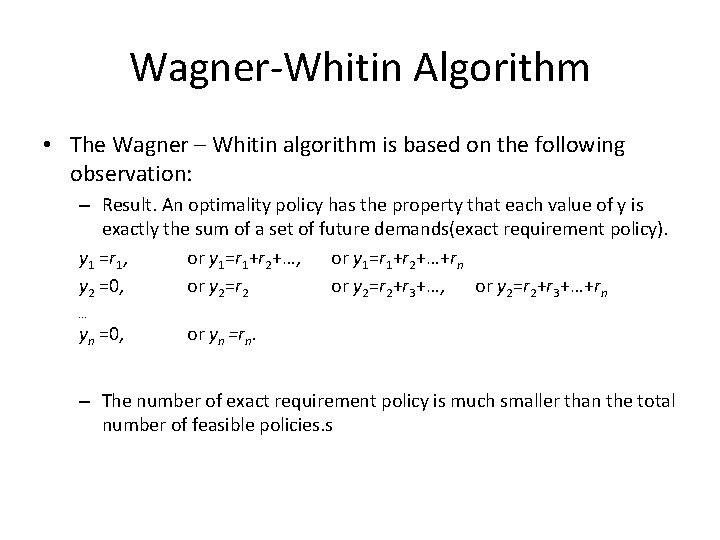
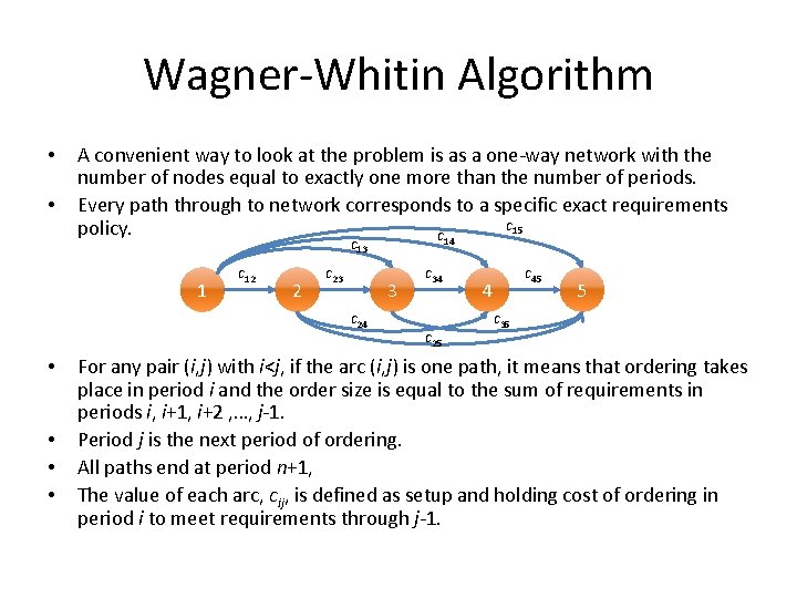
Wagner-Whitin Algorithm • The Wagner – Whitin algorithm is based on the following observation: – Result. An optimality policy has the property that each value of y is exactly the sum of a set of future demands(exact requirement policy). y 1 =r 1, or y 1=r 1+r 2+…+rn y 2 =0, or y 2=r 2+r 3+…, or y 2=r 2+r 3+…+rn … yn =0, or yn =rn. – The number of exact requirement policy is much smaller than the total number of feasible policies. s

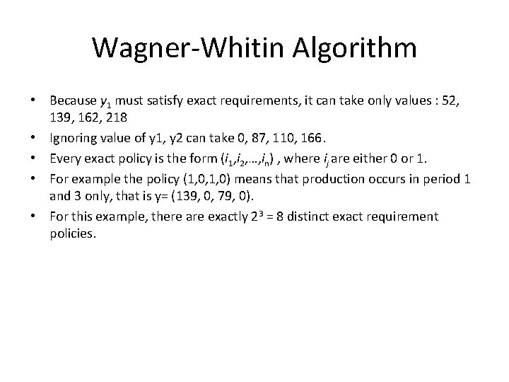
Wagner-Whitin Algorithm • Because y 1 must satisfy exact requirements, it can take only values : 52, 139, 162, 218 • Ignoring value of y 1, y 2 can take 0, 87, 110, 166. • Every exact policy is the form (i 1, i 2, …, in) , where ij are either 0 or 1. • For example the policy (1, 0, 1, 0) means that production occurs in period 1 and 3 only, that is y= (139, 0, 79, 0). • For this example, there are exactly 23 = 8 distinct exact requirement policies.

Wagner-Whitin Algorithm • • A convenient way to look at the problem is as a one-way network with the number of nodes equal to exactly one more than the number of periods. Every path through to network corresponds to a specific exact requirements c 15 policy. c 14 c 13 1 c 12 2 c 23 3 c 24 • • c 34 c 25 c 45 4 5 c 35 For any pair (i, j) with i<j, if the arc (i, j) is one path, it means that ordering takes place in period i and the order size is equal to the sum of requirements in periods i, i+1, i+2 , …, j-1. Period j is the next period of ordering. All paths end at period n+1, The value of each arc, cij, is defined as setup and holding cost of ordering in period i to meet requirements through j-1.

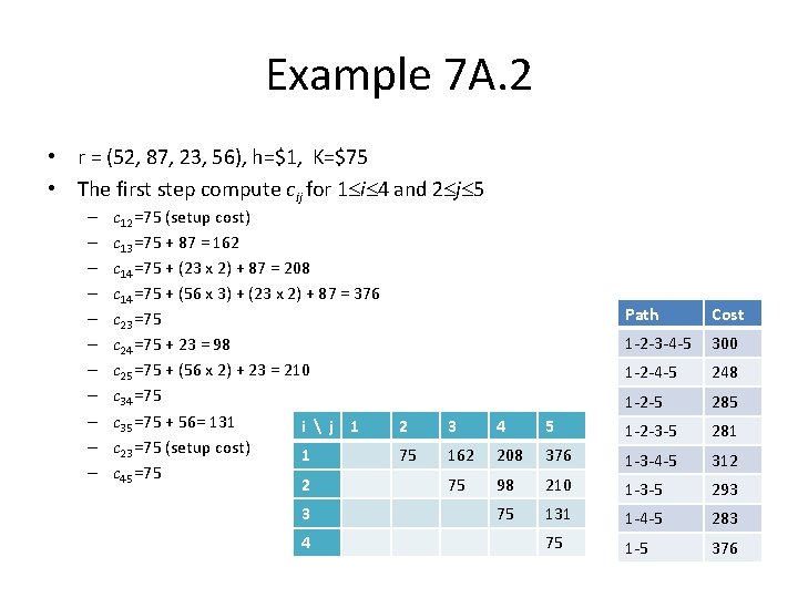
Example 7 A. 2 • r = (52, 87, 23, 56), h=$1, K=$75 • The first step compute cij for 1 i 4 and 2 j 5 – – – c 12 =75 (setup cost) c 13 =75 + 87 = 162 c 14 =75 + (23 x 2) + 87 = 208 c 14 =75 + (56 x 3) + (23 x 2) + 87 = 376 c 23 =75 c 24 =75 + 23 = 98 c 25 =75 + (56 x 2) + 23 = 210 c 34 =75 c 35 =75 + 56= 131 i j 1 c 23 =75 (setup cost) 1 c 45 =75 2 3 4 Path Cost 1 -2 -3 -4 -5 300 1 -2 -4 -5 248 1 -2 -5 285 2 3 4 5 1 -2 -3 -5 281 75 162 208 376 1 -3 -4 -5 312 75 98 210 1 -3 -5 293 75 131 1 -4 -5 283 75 1 -5 376

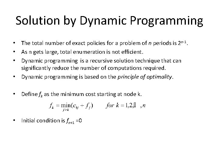
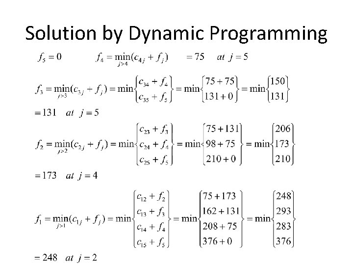
Solution by Dynamic Programming • The total number of exact policies for a problem of n periods is 2 n-1. • As n gets large, total enumeration is not efficient. • Dynamic programming is a recursive solution technique that can significantly reduce the number of computations required. • Dynamic programming is based on the principle of optimality. • Define fk as the minimum cost starting at node k. • Initial condition is fn+1 =0

Solution by Dynamic Programming