A snapshot of the 3 D magnetic field

A snapshot of the 3 D magnetic field structure simulated with the Glatzmaier-Roberts geodynamo model. Magnetic field lines are blue where the field is directed inward and yellow where directed outward. The rotation axis of the model Earth is vertical and through the center. A transition occurs at the core -mantle boundary from the intense, complicated field structure in the fluid core, where the field is generated, to the smooth, potential field structure outside the core. The field lines are drawn out to two Earth radii. Magnetic field is wrapped around the "tangent cylinder" due to the shear of the zonal fluid flow.

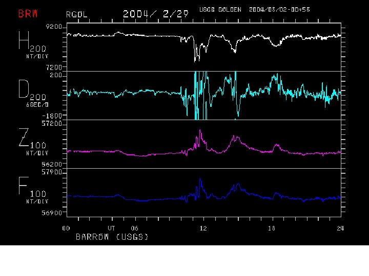
View online magnetograms from USGS geomagnetic observatories

Local view of the relationships of the geomagnetic field vector seen at the site of measurement. Shown is the total field H, the declination angle, D, measured in the horizontal plane, and the inclination angle, I, measured in the vertical plane. D is measured clockwise with respect to geographic north. SITE

North Pole (NP) This is the longitudinal great circle that passes through the North Pole and the observation site Red grid: geomagnetic latitudes and longitudes about geomagnetic north pole (shown as VGP here) This is the great circle through the observation site and the VGP; it is the same great circle shown in sections in the preceding figures. SITE Black grid: geographic latitudes and longitudes

Pointing in the direction of geographic North, along the great circle joining site and North Pole Pointing in the direction of magnetic North, along the great circle joining site and geomagnetic North Pole (VGP in diagrams) SITE

North Pole (NP) Thus from measurements of D and I at the site, one can 1) determine the great circle through the site which makes an angle, D, with the longitudinal great circle through the site; 2) measure the angular distance q, calculated from I, along the segment of the great circle (shown in red) connecting the SITE and the VGP. This determines the location of the “Virtual Geomagnetic Pole” or VGP which is the location of north geomagnetic pole assuming that the declination and inclination at the site result from a simple earth centered dipole.

Locations of the north pole of the dipole component of the geomagnetic field from 1600 2001. Canadian geomagnetic program: http: //www. geolab. nrcan. gc. ca/geomag/northpole_e. shtml

Locations of the north pole of the dipole component of the geomagnetic field from 1904 -2001. Magnetic field “jerks” Canadian geomagnetic program: http: //www. geolab. nrcan. gc. ca/geomag/northpole_e. shtml

Paleosecular poles from western US volcanic rocks Hagstrum and Champion, 2002, A Holocene paleosecular variation record from 14 C-dated volcanic rocks in western North America, J. Geophys. Res. , v. 107, B 1.

Summary of “continuous” data -30 to 3690 BP Average pole position for all data (94 poles): 88. 4 N 23. 8 W 1. 6 degrees from geographic North Pole -30 to 800 BP 800 to 1940 BP 1940 to 3690 BP Calibrated radiocarbon years before present, (B. P, AD 1950=0)

VGP’s determined for magnetized rocks less than 5 Ma modern geomagnetic pole

90 E 180 VGP’s average Earth’s rotation axis! Polar projection showing VGP’s derived from magnetization of igneous rocks at many sites, all dated at less than 20 million years old (too young to be significantly affected by plate motions). geographic North Pole 0 30 N 15 N 90 W

500 yrs before middle of reversal 500 yrs after “About 36, 000 years into the simulation the magnetic field underwent a reversal of its dipole moment (Figure 3), over a period of a little more than a thousand years. The intensity of the magnetic dipole moment decreased by about a factor of ten during the reversal and recovered immediately after, similar to what is seen in the Earth's paleomagnetic reversal record. ” (See mag_field. ppt for the source of the models shown above)

Excursions and transitions Excursions

Reversal rate, per Ma: Superchrons

Magnetizations (DRM) recovered from deep ocean sediments

Magnetizations (DRM) recovered from deep ocean sediments Note minimum intensities during reversals

Reversal captured in Columbia River basalt flows ( Steens Mtn. , Oregon: Miocene, 15. 5 Ma)

Steens Mtn: Kiger Gorge from the Steens Mountain Loop Road

High resolution record of geomagnetic field reversal Extrusions at rate of about 43 m/1000 yrs 3500 yrs 3600 yrs 5000 yrs Mankinen, et al. , 1985, J. Geophys. Res. , v. 90, p, 10400

Steens Mtn results: VGP’s in time

Figure 5 Spatial patterns of large-scale mantle and core dynamical structures. a, Map showing spatial distribution of subducted slabs that are expected to have penetrated to the base of the mantle (blue lines) and buoyancy flux weighted hotspots (red dots). b, Map showing virtual geomagnetic pole (VGP) reversal paths (green lines). To first order, reversal paths and hotspots appear to be anti-correlated, with reversal paths generally following approximately longitudinal bands in which the ULVZ has not been observed to be present