The Earths magnetic field The Earths magnetic field

The Earth’s magnetic field

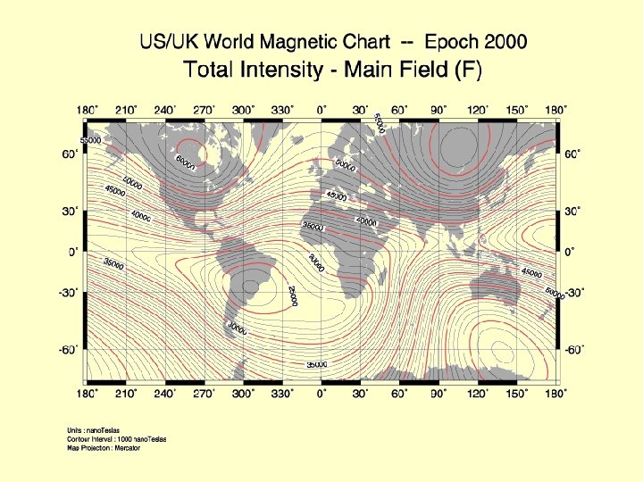
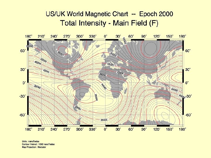
The Earth’s magnetic field The Earth's magnetic field crudely resembles that of a central dipole. On the Earth's surface the field varies from being horizontal and of magnitude about 30 000 n. T near the equator to vertical and about 60 000 n. T near the poles; the root mean square (rms) magnitude of the vector over the surface is about 45 000 n. T. The internal geomagnetic field also varies in time, on a time-scale of months and longer, in an as yet unpredictable manner. This so-called secular variation (SV) has a complicated spatial pattern, with a global rms magnitude of about 80 n. T/year.

Secular Variation of the dipole axis represented by the location of the North Geomagnetic Pole. (After Fraser-Smith, 1987)

Secular Variation of the dipole moment from successive spherical harmonic analyses. (After Fraser-Smith, 1987)

Secular Variation Play Shockwave Movies

The Earth’s magnetic field Consequently, any numerical model of the geomagnetic field has to have coefficients which vary with time. These coefficients are computed from observations from geomagnetic observatories that are distributed throughout the world, and from satellite observations (Magsat which flew in 197980, and the current Ørsted mission). They are usually updated every 5 years to produce the International Geomagnetic Reference Field (IGRF). The IGRF is a series of mathematical models describing the Earth’s main field and its secular variation.

The Earth’s magnetic field Each model comprises a set of spherical harmonic coefficients (called Gauss coefficients in recognition of Gauss’s development of this technique for geomagnetism), in a truncated series expansion of a geomagnetic potential function: where is the geomagnetic potential, a is the mean radius of the Earth (6371. 2 km) and r, , , are the geocentric spherical coordinates (r is the distance from the centre of the Earth, is the longitude eastward from Greenwich and is the colatitude (90° minus the latitude). 0 is the permeability of free space.

The Earth’s magnetic field The terms are Schmidt quasinormalized associated Legendre functions of degree n and order m (n 1 and m n). This gives values for the coefficients in nano-Tesla (n. T). The maximum spherical harmonic degree of the expansion is N.

The Earth’s magnetic field The IGRF models for the main field are truncated at N=10 (120 coefficients) which represents a compromise adopted to produce well-determined main-field models while avoiding most of the contamination resulting from crustal sources. The coefficients of the main field are rounded to the nearest nano. Tesla (n. T) to reflect the limit of the resolution of the available data. The IGRF models for the secular variation are truncated at N=8 (80 coefficients). This time the coefficients are rounded at the nearest 0. 1 n. T/year, this time to reduce the effect of accumulated rounding error.

The Earth’s magnetic field The main terms of interest in the above are the harmonics of order 0, which are zonal harmonics. Coefficents , , , are the coefficients of the geocentric axial dipole, the geocentric axial quadrupole, and the geocentric axial octupole respectively. The other coefficients are non-zonal, the major one of interest being the equatorial dipole ( , ), which causes the main dipole to be inclined to the axis of rotation by about 10. 5°.

The Earth’s magnetic field Some low-degree Legendre functions. Functions P 0( ) to P 6( ) are shown in the interval – 1< < 1.

The Earth’s magnetic field Surface projection of the geocentric axial dipole term. Yellow region indicates a downward pointing field and green indicates an upward pointing field.

The Earth’s magnetic field The main terms of interest in the above are the harmonics of order 0, which are zonal harmonics. Coefficents , , , are the coefficients of the geocentric axial dipole, the geocentric axial quadrupole, and the geocentric axial octupole respectively. The other coefficients are non-zonal, the major one of interest being the equatorial dipole ( , ), which causes the main dipole to be inclined to the axis of rotation by about 10. 5°.

The Earth’s magnetic field Some low-degree Legendre functions. Functions P 0( ) to P 6( ) are shown in the interval – 1< < 1.

The Earth’s magnetic field Surface projection of the geocentric axial quadrupole term. Yellow region indicates a downward pointing field and green indicates an upward pointing field.

The Earth’s magnetic field The main terms of interest in the above are the harmonics of order 0, which are zonal harmonics. Coefficents , , , are the coefficients of the geocentric axial dipole, the geocentric axial quadrupole, and the geocentric axial octupole respectively. The other coefficients are non-zonal, the major one of interest being the equatorial dipole ( , ), which causes the main dipole to be inclined to the axis of rotation by about 10. 5°.

The Earth’s magnetic field Some low-degree Legendre functions. Functions P 0( ) to P 6( ) are shown in the interval – 1< < 1.

The Earth’s magnetic field Surface projection of the geocentric axial octupole term. Yellow region indicates a downward pointing field and green indicates an upward pointing field.

The Earth’s magnetic field The main terms of interest in the above are the harmonics of order 0, which are zonal harmonics. Coefficents , , , are the coefficients of the geocentric axial dipole, the geocentric axial quadrupole, and the geocentric axial octupole respectively. The other coefficients are non-zonal, the major one of interest being the equatorial dipole ( , ), which causes the main dipole to be inclined to the axis of rotation by about 10. 5°.

The Earth’s magnetic field Surface projection of the equatorial dipole term. Yellow region indicates a downward pointing field and green indicates an upward pointing field.

The Earth’s magnetic field

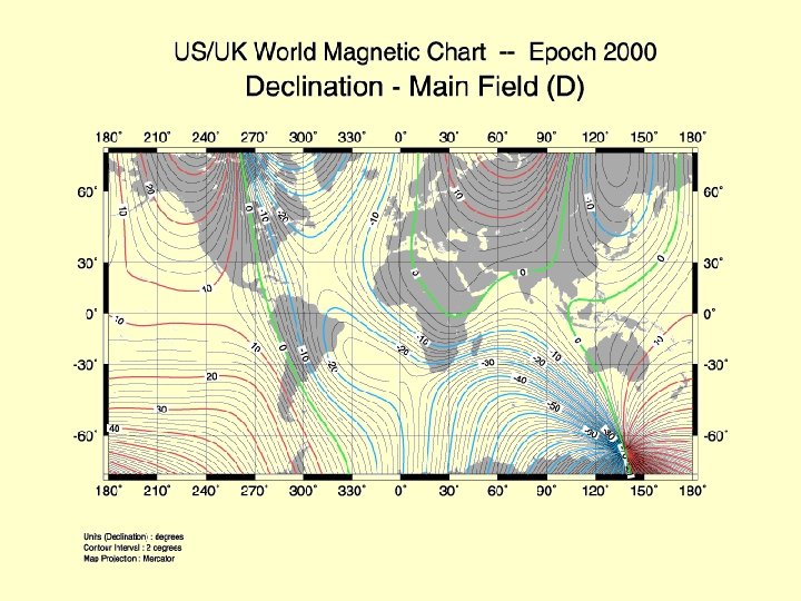
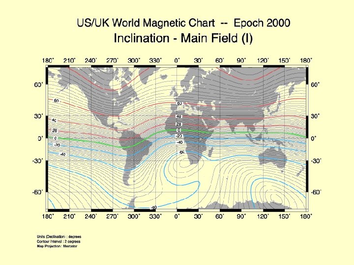
The Earth’s magnetic field I = +90 o I = -90 o This variation on timescales of decades to hundreds or years is known as secular variation. When averaged over time scaled of several thousands of years the magnetic field resembles that of a dipole, where there is a simple relationship between latitude and the inclination of the Earth’s magnetic field: Tan I = 2 Tan l

Generation of the Earth’s magnetic field The dynamo theory of the Earth’s magnetic field originates from papers by Elasser and Bullard in the 1940’s that the electrically conducting core of the Earth acts like a self-exciting dynamo, and produces the electrical currents needed to sustain the field. The solution of this idea in an Earth-like scenario has, however, proven to be very difficult. This is because the Earth has a homogenous, highly electrically conductive, rapidly rotating, convecting fluid that forms the dynamo. Thus the equations needed to provide a solution to the generation of the field are, of necessity, fluid dynamical ones. With the advent of more powerful supercomputers major advances have been made in recent years.

Why does the Earth have a magnetic field? The Earth has, at its centre, a dense liquid core, of about half the radius of the Earth, with a solid inner core. This core is though to be mostly made of molten iron, perhaps mixed with some lighter elements. The Earth's magnetic field is generated by fluid motions in the Earth's core, from circulating flows that help get rid of heat produced there. The source of this heat is poorly understood: it might come from some of the iron becoming solid and joining the inner core, releasing latent heat, or perhaps it is generated by radioactivity, like the heat of the Earth's crust. The circulation of the molten iron in the outer core is very slow, and the energy involved is just a tiny part of the total heat energy contained in the core. By moving through the existing magnetic field, the molten iron creates a system of electric currents, spread out through the core. These currents create the magnetic field.

Generation of the Earth’s magnetic field A number of concepts are central to the understanding of the geodynamo: Frozen-in-field theorem: If a magnetic field exists in a perfectly conducting medium, the magnetic field lines be carried along with the fluid medium. This is a central concept because it means that the differential motions of the fluid stretch the field lines and add energy to the field. In the case of the Earth, however, the fluid is not a perfect conductor and the magnetic field will therefore diffuse away with time. To overcome this diffusion dynamo action is necessary to add energy back into the system.

Generation of the Earth’s magnetic field Poloidal and Toroidal fields: Toroidal fields have no radial component and cannot, therefore, be observed at the earth’s surface whereas poloidal fields do have a radial component. The geomagnetic field at the Earth’s surface is therefore poloidal. A central issue in geodynamo models is how it’s possible to generate a toroidal field from a poloidal one and vice-versa as the feed-backs between the two provide the necessary energy to maintain the geodynamo.

Generation of the Earth’s magnetic field Production of a toroidal magnetic field in the core: w-model a) an initial poloidal field passing through the Earth’s core is subjected to an initial cylindrical shear motion of the fluid. b) The fluid motion ‘drags’ out the magnetic field lines, and after one complete circuit we have generated 2 new toroidal loops of opposite sign. (After Parker, 1955)

Generation of the Earth’s magnetic field Poloidal and Toroidal fields: Toroidal fields have no radial component and cannot, therefore, be observed at the earth’s surface whereas poloidal fields do have a radial component. The geomagnetic field at the Earth’s surface is therefore poloidal. A central issue in geodynamo models is how it’s possible to generate a toroidal field from a poloidal one and vice-versa as the feed-backs between the two provide the necessary energy to maintain the geodynamo.

Generation of the Earth’s magnetic field Rotation due to Coriolis force (anticlockwise in Northern Hemisphere) = Helicity Production of a poloidal magnetic field in the northern hemisphere: a-model A region of fluid upwelling interacts with the field line. Because of the Coriolis force the fluid exhibits helicity (rotating as it moves upwards). The magnetic field line is carried along and twisted to produce a poloidal loop. (After Parker, 1955)

The Alpha – Omega Dynamo Cycle Consider an initial dipolar poloidal field, such as in (a). The omega-effect consists of (b, c) differential rotation, wrapping the magnetic field around the rotational axis, thereby creating (d) a quadrupolar toroidal field magnetic field inside the core. A closure of the dynamo cycle requires a bit of symmetry breaking, brought about by the alpha-effect, whereby (e) helical upwelling and downwelling creates loops of magnetic field. These loops coalesce (f) to reinforce the original dipolar field.

Why does the Earth have a magnetic field? Because the Earth is spinning the convection in the outer core is influenced by the motion of the planet. The picture on the right depicts region where fluid The flows form an imaginary “tangent flow is greatest within the outer core cylinder” due to the effects of large (the core-mantle boundary is the blue rotation, small fluid viscosity and the mesh; and the inner-outer core presence of a solid inner core within the boundary is the red mesh). spherical shell of the outer core.

Why does the Earth have a magnetic field? Because the flow lines within the outer core form a ‘tangent cylinder’ the magnetic field lines generated also tend to wrap around the inner core. On the left is depicted a snapshot of the 3 D magnetic field structure simulated with a computer generated field model. Magnetic field lines are blue where the field is directed inward and yellow where directed outward. The rotation axis of the model Earth is vertical and through the centre. A transition occurs at the core-mantle boundary from the intense, complicated field structure in the fluid core, where the field is generated, to the smooth, potential field structure outside the core. The field lines are drawn out to two Earth radii. The magnetic field is wrapped around the “tangent cylinder” due to the shear of the zonal fluid flow.

Reversals of the field The Earths magnetic field is known to have reversed its polarity in the past: that is the magnetic field has “flipped” to flow from North to South. These reversals are not periodic and episodes of constant polarity vary greatly in length. The history of reversals of the Earths magnetic field is very well known for the past 200 million years. Magnetostratigraphy involves measuring the pattern of reversals in a sequence of rocks. This yields a unique fingerprint, or “barcode”, of reversals that can be matched to known reversal records elsewhere. This fingerprint can be used to date rocks and in correlating different rock sequences.

Why does it reverse? Because the field is generated by fluid flow the geometry of the field is affected by any instabilities within the flow. The field is time varying, but polarity is stabilised by the presence of an inner core. Any field reversal must reverse the field in the inner core and the inner core therefore damps the effect of any turbulence in flow in the outer core. If instabilities build up for a long enough period of time the flow can induce the opposite polarity and hence we have a reversal.

How does it reverse? A full understanding of how the field reverses has yet to be achieved. Two main approaches are currently being used to study how the field reverses. The first is the study of the behaviour of the field through the magnetic records preserved in rock sequences. However to get a full 3 -d picture of what happens multiple studies of the same reversal are required from multiple sites spread out around the globe. This will take some time to achieve. The second approach is the use of supercomputers to model the behaviour of the field through time. The model on the left depicts a reversal in the computer model of Glatzmaier & Roberts (1995). Note that the field lines become chaotic during the reversal but revert to a dipole geometry once the reversal is complete.

How does it reverse? A snapshot of the 3 D magnetic field structure simulated with the Glatzmaier-Roberts geodynamo model. Magnetic field lines are blue where the field is directed inward and yellow where directed outward. The rotation axis of the model Earth is vertical and through the centre. A transition occurs at the core-mantle boundary from the intense, complicated field structure in the fluid core, where the field is generated, to the smooth, potential field structure outside the core. The field lines are drawn out to two Earth radii. Magnetic field is wrapped around the “tangent cylinder” due to the shear of the zonal fluid flow.

How does it reverse? 500 years before the middle of a magnetic reversal.

How does it reverse? During the middle of a magnetic reversal

How does it reverse? 500 years after the middle of a magnetic reversal

How does it reverse? A snapshot of the simulated magnetic field structure within the core. Lines are blue where outside the inner core and orange within the inner core. The rotation axis is vertical.

Preferred Reversal Paths? Transitional VGP paths for the upper Olduvai transition in the Cristolo sediment. 362 transitional VGPs from 121 volcanic record of reversals younger than 16 Ma. After: Tric et al. , 1991; Prevot & Camps, 1993

Preferred Reversal Paths? Equator crossings for sedimentary VGP transition paths up to 1995. After: Mc. Fadden & Merrill, (1995)

What triggers reversals?

Polarity Lengths and Superchrons

Non-Dipole Fields in the Past? A fundamental assumption in all plate reconstructions based on magnetic data is that we are dealing with a time-averaged geocentric axial dipole. (Kent & Smethurst 1998)

Non-Dipole Fields in the Past? The addition of varying proportions of non-dipole fields will have the effect of changing the inclination vs latitude relationship: Tan I = 2 Tan l. Here the addition of quadrupole fields is modelled. (Kent & Smethurst 1998)

Non-Dipole Fields in the Past? The addition of varying proportions of non-dipole fields will have the effect of changing the inclination vs latitude relationship: Tan I = 2 Tan l. Here the addition of octupole fields is modelled. After Kent & Smethurst 1998.

Non-Dipole Fields in the Past? The Frequency vs Inclination distribution for Palaeozoic Rocks is far from dipolar. This could indicate: • Non-dipole fields • Shallowing of inclinations in sedimentary sequences • Inadequate global sampling (i. e. – we just happen to have sampled the lowlatitude continents) After Kent & Smethurst 1998.

Non-Dipole Fields in the Past? It is possible to model the distributions in terms of non-dipole contributions to the main field. After Kent & Smethurst 1998.