9 1 Chapter Nine Comparing Population Means 9

9 -1

Chapter Nine Comparing Population Means 9 -2 Mc. Graw-Hill/Irwin Copyright © 2004 by The Mc. Graw-Hill Companies, Inc. All rights reserved.

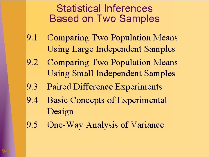
Statistical Inferences Based on Two Samples 9. 1 9. 2 9. 3 9. 4 9. 5 9 -3 Comparing Two Population Means Using Large Independent Samples Comparing Two Population Means Using Small Independent Samples Paired Difference Experiments Basic Concepts of Experimental Design One-Way Analysis of Variance

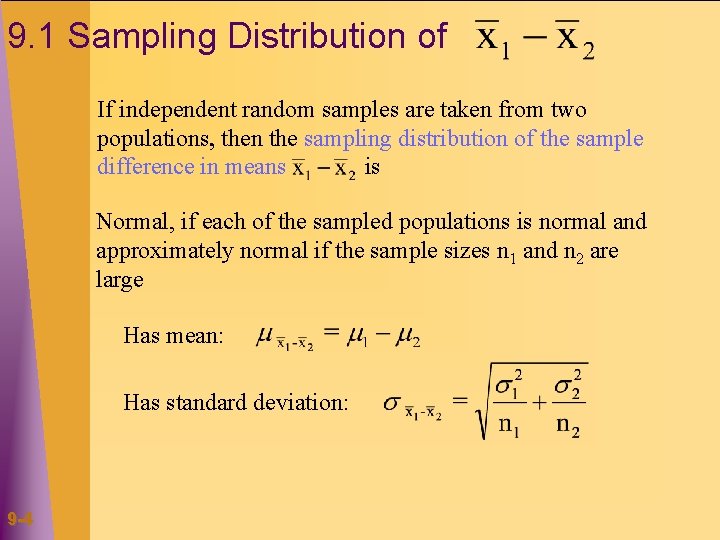
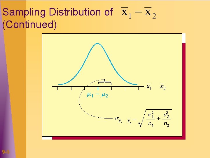
9. 1 Sampling Distribution of If independent random samples are taken from two populations then the sampling distribution of the sample difference in means is Normal, if each of the sampled populations is normal and approximately normal if the sample sizes n 1 and n 2 are large Has mean: Has standard deviation: 9 -4

Sampling Distribution of (Continued) 9 -5

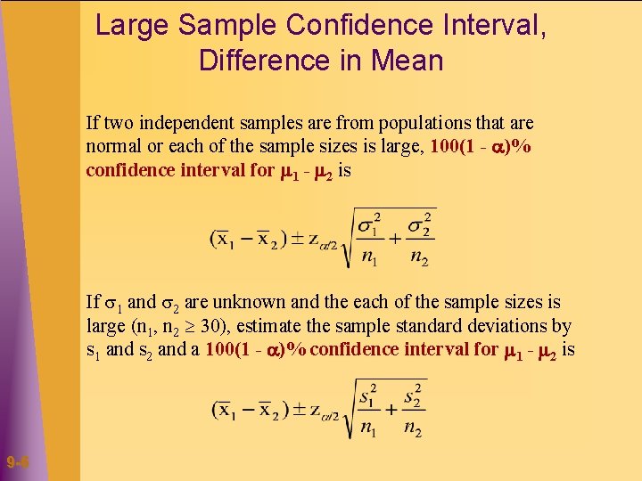
Large Sample Confidence Interval, Difference in Mean If two independent samples are from populations that are normal or each of the sample sizes is large, 100(1 - )% confidence interval for 1 - 2 is If 1 and 2 are unknown and the each of the sample sizes is large (n 1, n 2 30), estimate the sample standard deviations by s 1 and s 2 and a 100(1 - )% confidence interval for 1 - 2 is 9 -6

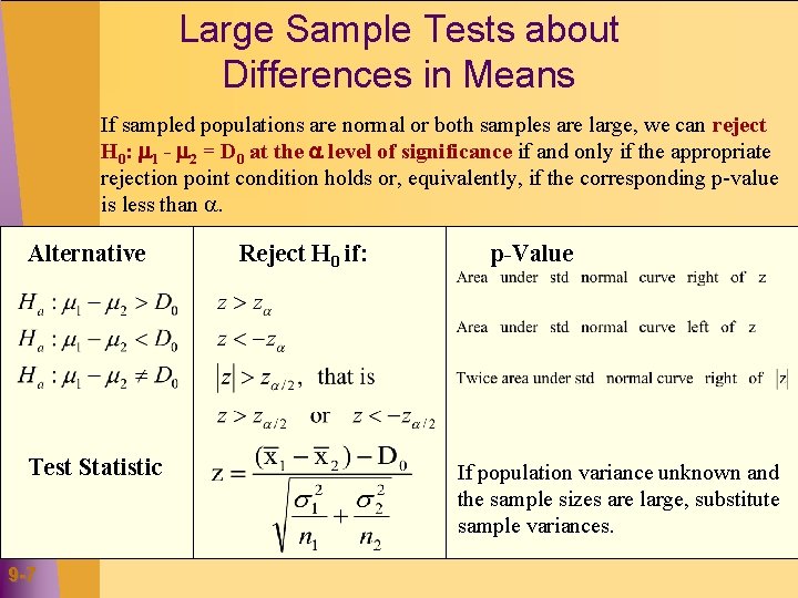
Large Sample Tests about Differences in Means If sampled populations are normal or both samples are large, we can reject H 0: 1 - 2 = D 0 at the level of significance if and only if the appropriate rejection point condition holds or, equivalently, if the corresponding p-value is less than . Alternative Test Statistic 9 -7 Reject H 0 if: p-Value If population variance unknown and the sample sizes are large, substitute sample variances.

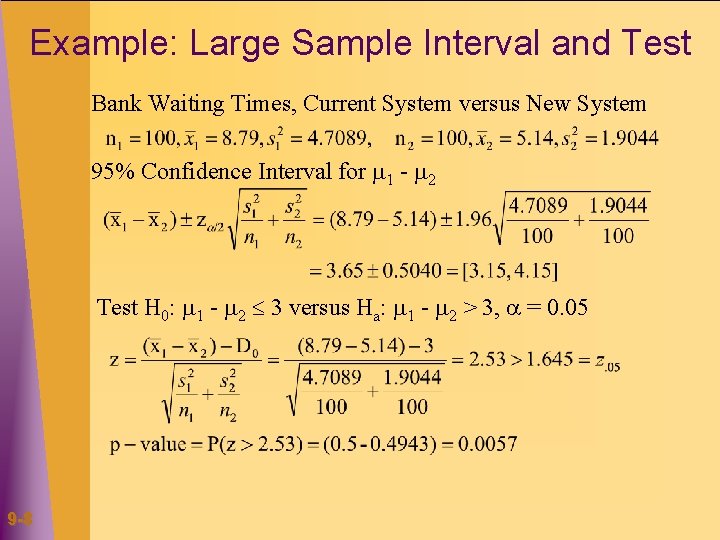
Example: Large Sample Interval and Test Bank Waiting Times, Current System versus New System 95% Confidence Interval for 1 - 2 Test H 0: 1 - 2 3 versus Ha: 1 - 2 > 3, = 0. 05 9 -8

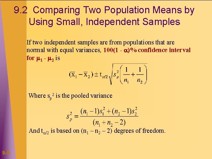
9. 2 Comparing Two Population Means by Using Small, Independent Samples If two independent samples are from populations that are normal with equal variances, 100(1 - )% confidence interval for 1 - 2 is Where sp 2 is the pooled variance And t /2 is based on (n 1 – n 2 – 2) degrees of freedom. 9 -9

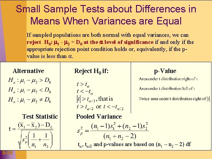
Small Sample Tests about Differences in Means When Variances are Equal If sampled populations are both normal with equal variances, we can reject H 0: 1 - 2 = D 0 at the level of significance if and only if the appropriate rejection point condition holds or, equivalently, if the pvalue is less than . Alternative Test Statistic Reject H 0 if: p-Value Pooled Variance t , t /2 and p-values are based on (n 1 – n 2 – 2) df 9 -10

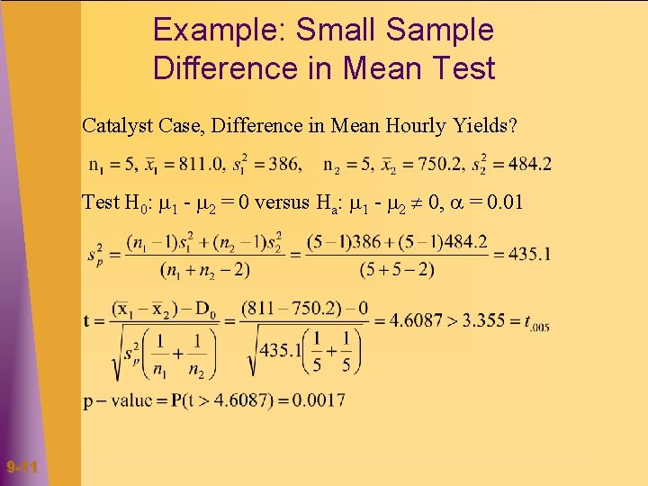
Example: Small Sample Difference in Mean Test Catalyst Case, Difference in Mean Hourly Yields? Test H 0: 1 - 2 = 0 versus Ha: 1 - 2 0, = 0. 01 9 -11

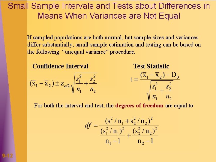
Small Sample Intervals and Tests about Differences in Means When Variances are Not Equal If sampled populations are both normal, but sample sizes and variances differ substantially, small-sample estimation and testing can be based on the following “unequal variance” procedure. Confidence Interval Test Statistic For both the interval and test, the degrees of freedom are equal to 9 -12

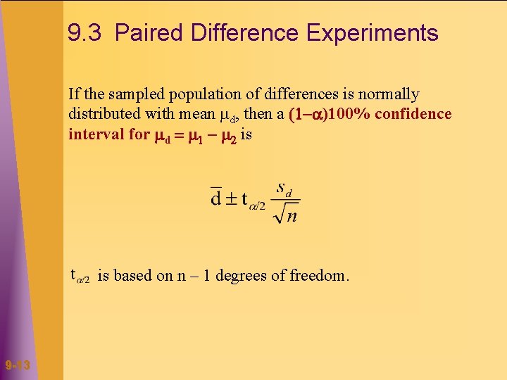
9. 3 Paired Difference Experiments If the sampled population of differences is normally distributed with mean d, then a (1 - )100% confidence interval for d = 1 - 2 is is based on n – 1 degrees of freedom. 9 -13

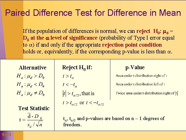
Paired Difference Test for Difference in Mean If the population of differences is normal, we can reject H 0: d = D 0 at the level of significance (probability of Type I error equal to ) if and only if the appropriate rejection point condition holds or, equivalently, if the corresponding p-value is less than . Alternative Reject H 0 if: p-Value Test Statistic t , t /2 and p-values are based on n – 1 degrees of freedom. 9 -14

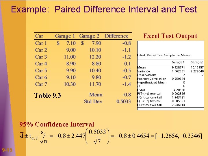
Example: Paired Difference Interval and Test Excel Test Output Table 9. 3 95% Confidence Interval 9 -15

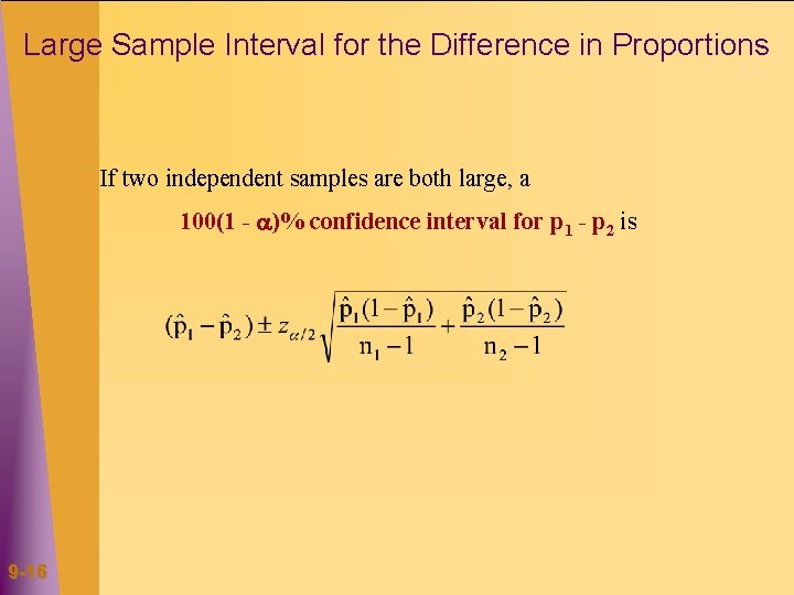
Large Sample Interval for the Difference in Proportions If two independent samples are both large, a 100(1 - )% confidence interval for p 1 - p 2 is 9 -16

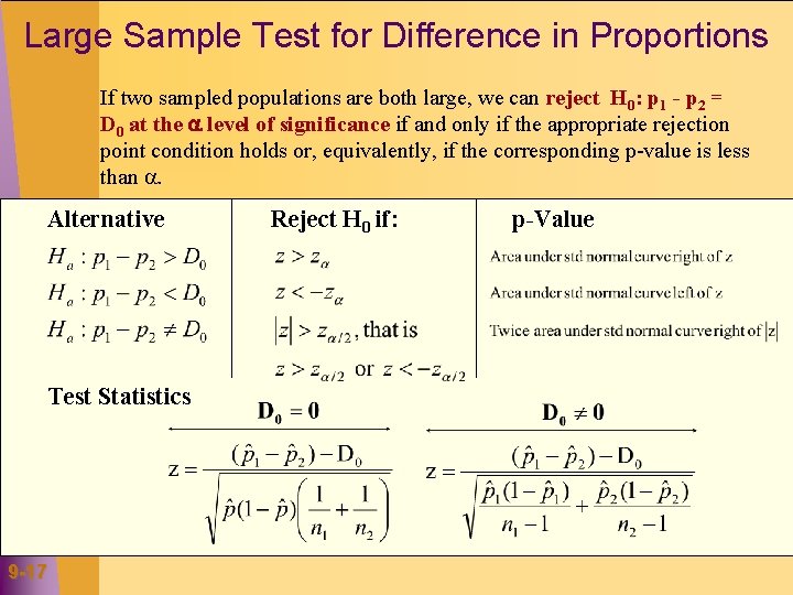
Large Sample Test for Difference in Proportions If two sampled populations are both large, we can reject H 0: p 1 - p 2 = D 0 at the level of significance if and only if the appropriate rejection point condition holds or, equivalently, if the corresponding p-value is less than . Alternative Test Statistics 9 -17 Reject H 0 if: p-Value

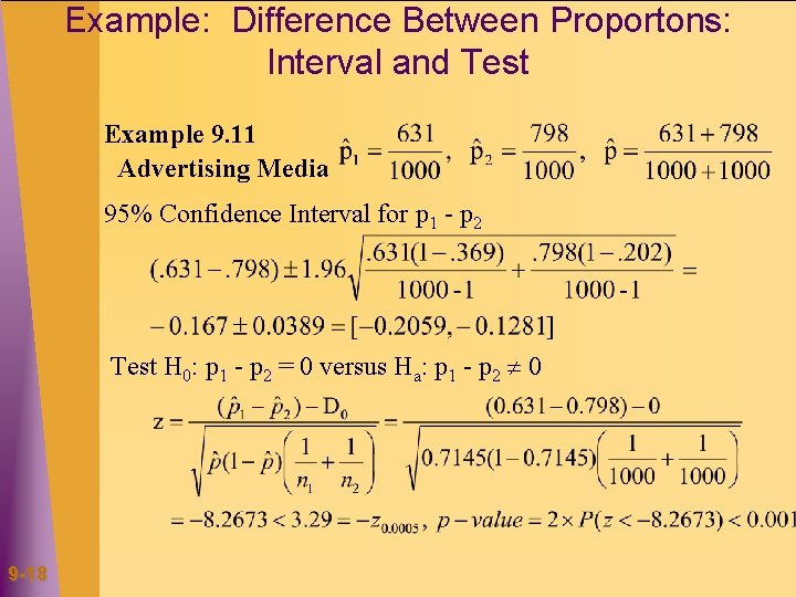
Example: Difference Between Proportons: Interval and Test Example 9. 11 Advertising Media 95% Confidence Interval for p 1 - p 2 Test H 0: p 1 - p 2 = 0 versus Ha: p 1 - p 2 0 9 -18

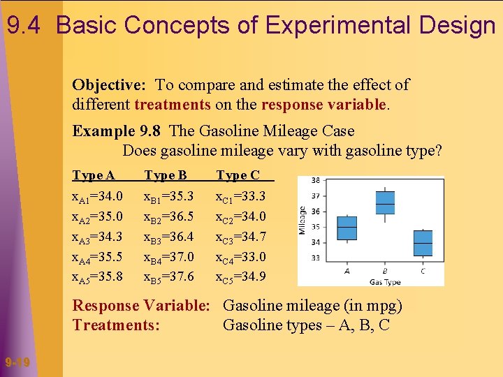
9. 4 Basic Concepts of Experimental Design Objective: To compare and estimate the effect of different treatments on the response variable. Example 9. 8 The Gasoline Mileage Case Does gasoline mileage vary with gasoline type? Type A Type B Type C x. A 1=34. 0 x. A 2=35. 0 x. A 3=34. 3 x. A 4=35. 5 x. A 5=35. 8 x. B 1=35. 3 x. B 2=36. 5 x. B 3=36. 4 x. B 4=37. 0 x. B 5=37. 6 x. C 1=33. 3 x. C 2=34. 0 x. C 3=34. 7 x. C 4=33. 0 x. C 5=34. 9 Response Variable: Gasoline mileage (in mpg) Treatments: Gasoline types – A, B, C 9 -19

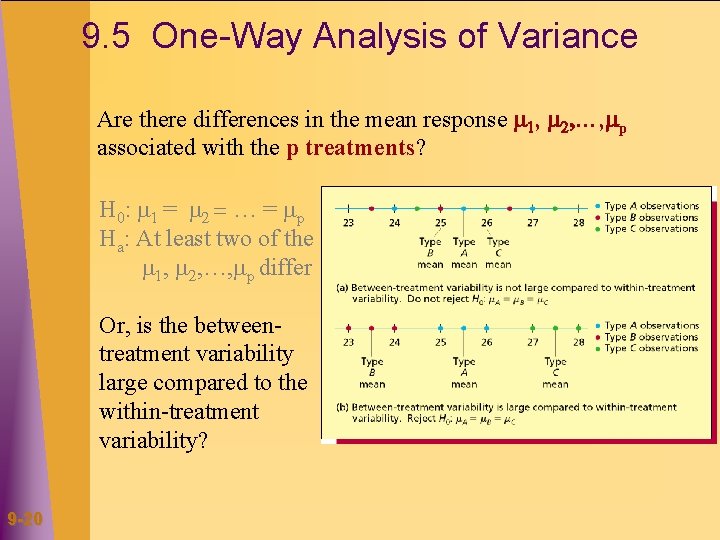
9. 5 One-Way Analysis of Variance Are there differences in the mean response 1, 2, …, p associated with the p treatments? H 0: 1 = 2 = … = p Ha: At least two of the 1, 2, …, p differ Or, is the betweentreatment variability large compared to the within-treatment variability? 9 -20

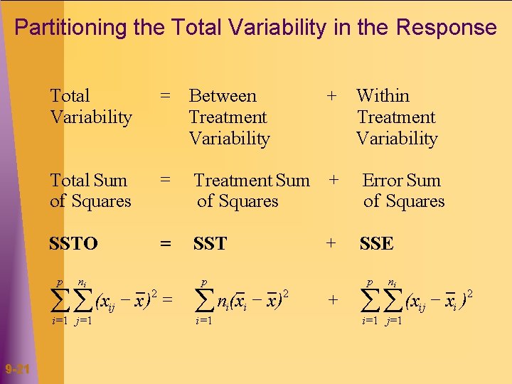
Partitioning the Total Variability in the Response Total Variability = Between Treatment Variability Total Sum of Squares = Treatment Sum + of Squares SSTO = SST p ni 2 = (x x ) åå ij i=1 j=1 9 -21 p 2 n ( x x ) åi i i=1 + Within Treatment Variability + + Error Sum of Squares SSE p ni 2 (x x ) åå ij i i=1 j=1

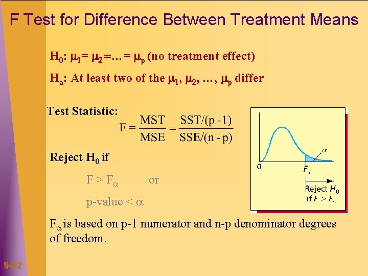
F Test for Difference Between Treatment Means H 0: 1= 2 =…= p (no treatment effect) Ha: At least two of the 1, 2, …, p differ Test Statistic: Reject H 0 if F > F or p-value < F is based on p-1 numerator and n-p denominator degrees of freedom. 9 -22

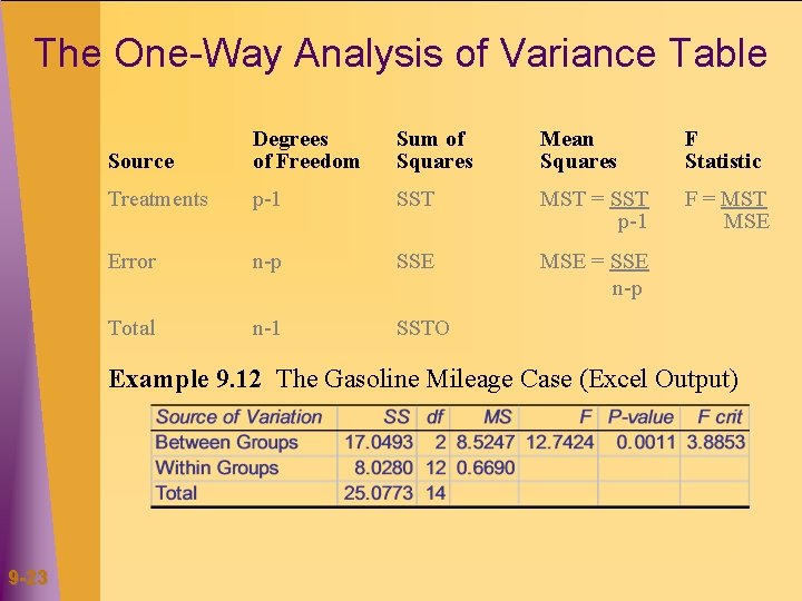
The One-Way Analysis of Variance Table Source Degrees of Freedom Sum of Squares Mean Squares F Statistic Treatments p-1 SST MST = SST p-1 F = MST MSE Error n-p SSE MSE = SSE n-p Total n-1 SSTO Example 9. 12 The Gasoline Mileage Case (Excel Output) 9 -23

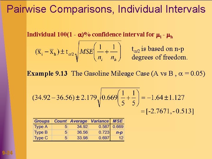
Pairwise Comparisons, Individual Intervals Individual 100(1 - )% confidence interval for i - h t /2 is based on n-p degrees of freedom. Example 9. 13 The Gasoline Mileage Case (A vs B , = 0. 05) 9 -24

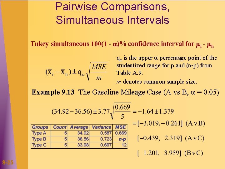
Pairwise Comparisons, Simultaneous Intervals Tukey simultaneous 100(1 - )% confidence interval for i - h q is the upper percentage point of the studentized range for p and (n-p) from Table A. 9. m denotes common sample size. Example 9. 13 The Gasoline Mileage Case (A vs B, = 0. 05) 9 -25

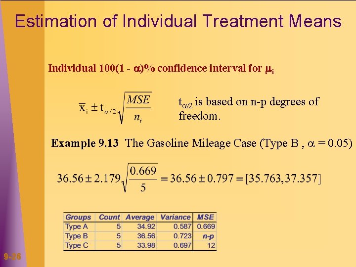
Estimation of Individual Treatment Means Individual 100(1 - )% confidence interval for i t /2 is based on n-p degrees of freedom. Example 9. 13 The Gasoline Mileage Case (Type B , = 0. 05) 9 -26

Statistical Inferences Based on Two Samples Summary: 9. 1 9. 2 9. 3 9. 4 9. 5 9 -27 Comparing Two Population Means Using Large Independent Samples Comparing Two Population Means Using Small Independent Samples Paired Difference Experiments Basic Concepts of Experimental Design One-Way Analysis of Variance