Chapter 5 Comparing 2 Population Means and Medians

Chapter 5 Comparing 2 Population Means and Medians

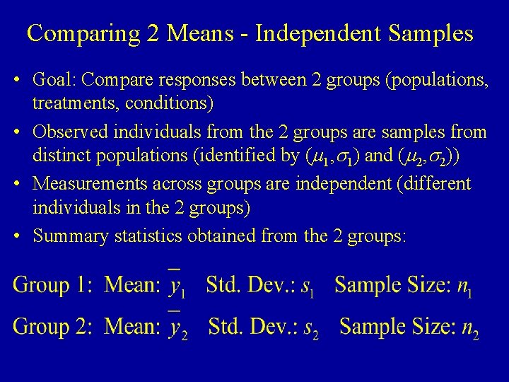
Comparing 2 Means - Independent Samples • Goal: Compare responses between 2 groups (populations, treatments, conditions) • Observed individuals from the 2 groups are samples from distinct populations (identified by (m 1, s 1) and (m 2, s 2)) • Measurements across groups are independent (different individuals in the 2 groups) • Summary statistics obtained from the 2 groups:

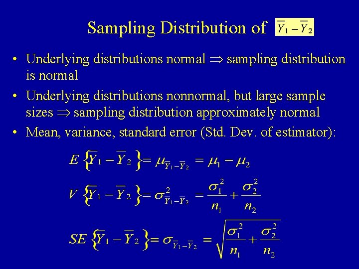
Sampling Distribution of • Underlying distributions normal sampling distribution is normal • Underlying distributions nonnormal, but large sample sizes sampling distribution approximately normal • Mean, variance, standard error (Std. Dev. of estimator):

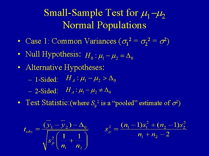
Small-Sample Test for m 1 -m 2 Normal Populations • Case 1: Common Variances (s 12 = s 2) • Null Hypothesis: • Alternative Hypotheses: – 1 -Sided: – 2 -Sided: • Test Statistic: (where Sp 2 is a “pooled” estimate of s 2)

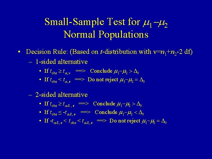
Small-Sample Test for m 1 -m 2 Normal Populations • Decision Rule: (Based on t-distribution with n=n 1+n 2 -2 df) – 1 -sided alternative • If tobs ta, n ==> Conclude m 1 -m 2 > D 0 • If tobs < ta, n ==> Do not reject m 1 -m 2 = D 0 – 2 -sided alternative • If tobs ta/2 , n ==> Conclude m 1 -m 2 > D 0 • If tobs ≤ -ta/2, n ==> Conclude m 1 -m 2 < D 0 • If -ta/2, n < tobs < ta/2, n ==> Do not reject m 1 -m 2 = D 0

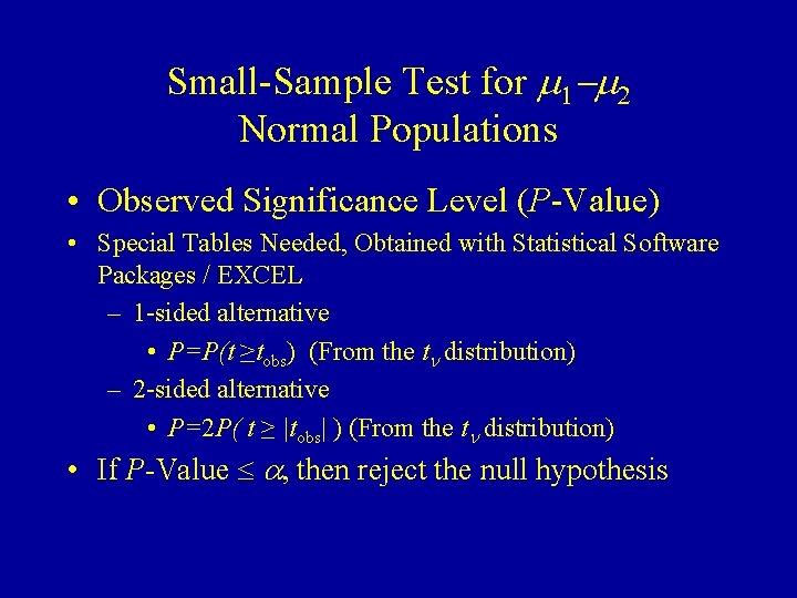
Small-Sample Test for m 1 -m 2 Normal Populations • Observed Significance Level (P-Value) • Special Tables Needed, Obtained with Statistical Software Packages / EXCEL – 1 -sided alternative • P=P(t ≥tobs) (From the tn distribution) – 2 -sided alternative • P=2 P( t ≥ |tobs| ) (From the tn distribution) • If P-Value a, then reject the null hypothesis

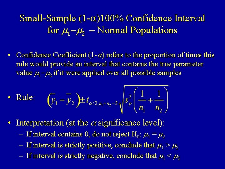
Small-Sample (1 -a)100% Confidence Interval for m 1 -m 2 - Normal Populations • Confidence Coefficient (1 -a) refers to the proportion of times this rule would provide an interval that contains the true parameter value m 1 -m 2 if it were applied over all possible samples • Rule: • Interpretation (at the a significance level): – If interval contains 0, do not reject H 0: m 1 = m 2 – If interval is strictly positive, conclude that m 1 > m 2 – If interval is strictly negative, conclude that m 1 < m 2

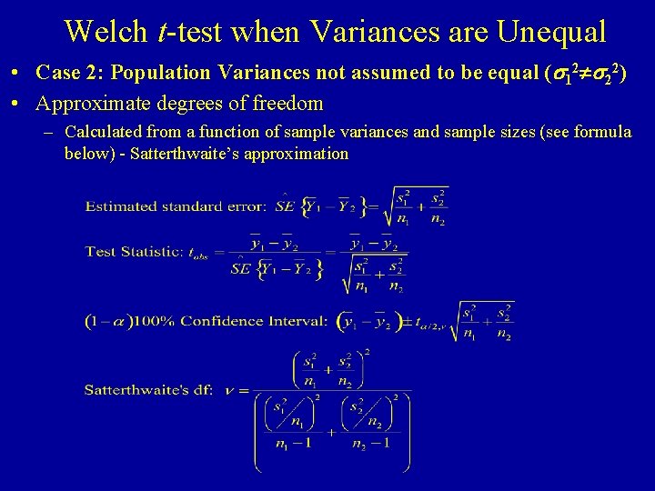
Welch t-test when Variances are Unequal • Case 2: Population Variances not assumed to be equal (s 12 s 22) • Approximate degrees of freedom – Calculated from a function of sample variances and sample sizes (see formula below) - Satterthwaite’s approximation

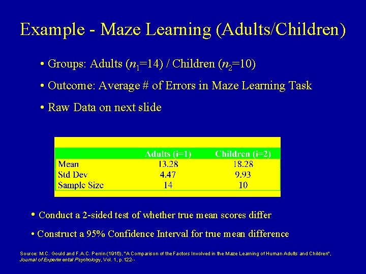
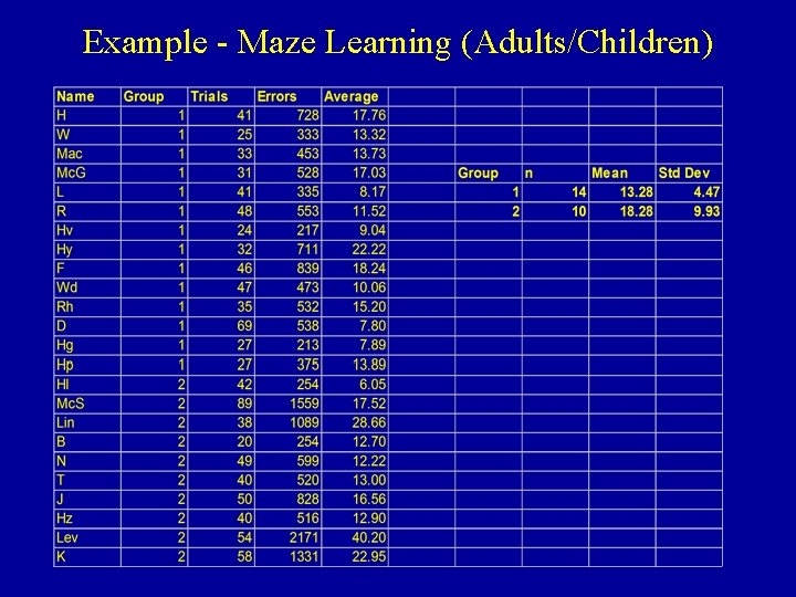
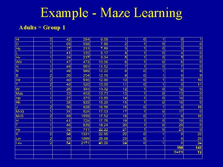
Example - Maze Learning (Adults/Children) • Groups: Adults (n 1=14) / Children (n 2=10) • Outcome: Average # of Errors in Maze Learning Task • Raw Data on next slide • Conduct a 2 -sided test of whether true mean scores differ • Construct a 95% Confidence Interval for true mean difference Source: M. C. Gould and F. A. C. Perrin (1916), "A Comparison of the Factors Involved in the Maze Learning of Human Adults and Children", Journal of Experimental Psychology, Vol. 1, p. 122 --

Example - Maze Learning (Adults/Children)

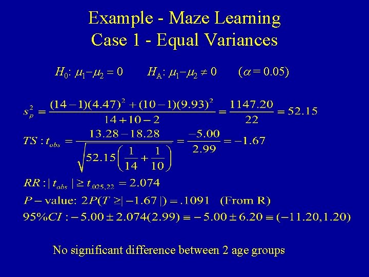
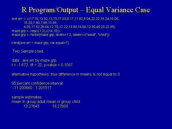
Example - Maze Learning Case 1 - Equal Variances H 0: m 1 -m 2 = 0 HA: m 1 -m 2 0 (a = 0. 05) No significant difference between 2 age groups

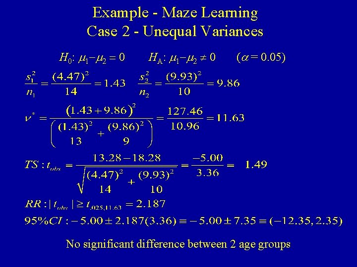
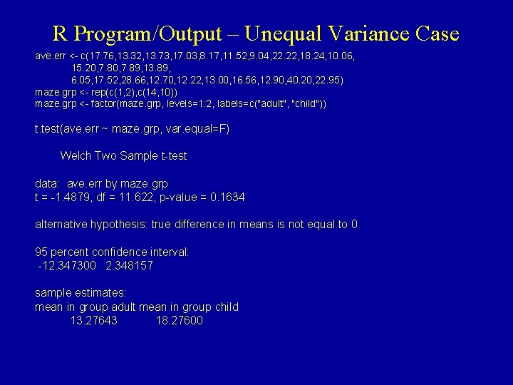
Example - Maze Learning Case 2 - Unequal Variances H 0: m 1 -m 2 = 0 HA: m 1 -m 2 0 (a = 0. 05) No significant difference between 2 age groups

R Program/Output – Equal Variance Case ave. err <- c(17. 76, 13. 32, 13. 73, 17. 03, 8. 17, 11. 52, 9. 04, 22. 22, 18. 24, 10. 06, 15. 20, 7. 89, 13. 89, 6. 05, 17. 52, 28. 66, 12. 70, 12. 22, 13. 00, 16. 56, 12. 90, 40. 20, 22. 95) maze. grp <- rep(c(1, 2), c(14, 10)) maze. grp <- factor(maze. grp, levels=1: 2, labels=c("adult", "child")) t. test(ave. err ~ maze. grp, var. equal=T) Two Sample t-test data: ave. err by maze. grp t = -1. 672, df = 22, p-value = 0. 1087 alternative hypothesis: true difference in means is not equal to 0 95 percent confidence interval: -11. 200660 1. 201517 sample estimates: mean in group adult mean in group child 13. 27643 18. 27600

R Program/Output – Unequal Variance Case ave. err <- c(17. 76, 13. 32, 13. 73, 17. 03, 8. 17, 11. 52, 9. 04, 22. 22, 18. 24, 10. 06, 15. 20, 7. 89, 13. 89, 6. 05, 17. 52, 28. 66, 12. 70, 12. 22, 13. 00, 16. 56, 12. 90, 40. 20, 22. 95) maze. grp <- rep(c(1, 2), c(14, 10)) maze. grp <- factor(maze. grp, levels=1: 2, labels=c("adult", "child")) t. test(ave. err ~ maze. grp, var. equal=F) Welch Two Sample t-test data: ave. err by maze. grp t = -1. 4879, df = 11. 622, p-value = 0. 1634 alternative hypothesis: true difference in means is not equal to 0 95 percent confidence interval: -12. 347300 2. 348157 sample estimates: mean in group adult mean in group child 13. 27643 18. 27600

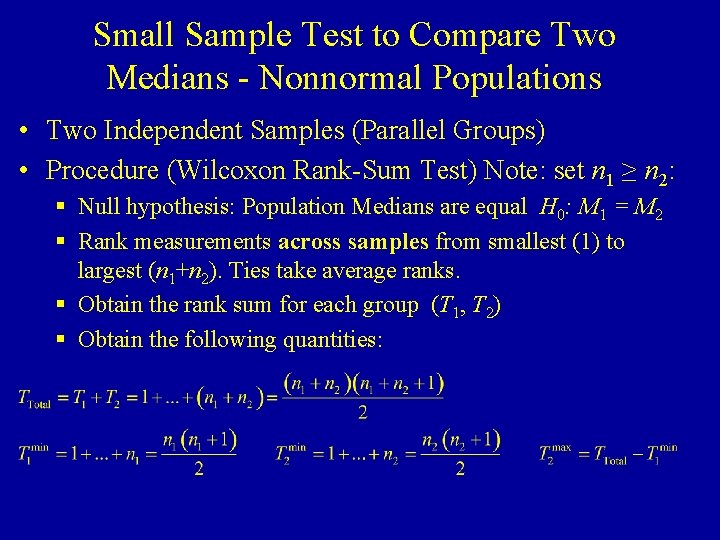
Small Sample Test to Compare Two Medians - Nonnormal Populations • Two Independent Samples (Parallel Groups) • Procedure (Wilcoxon Rank-Sum Test) Note: set n 1 ≥ n 2: § Null hypothesis: Population Medians are equal H 0: M 1 = M 2 § Rank measurements across samples from smallest (1) to largest (n 1+n 2). Ties take average ranks. § Obtain the rank sum for each group (T 1, T 2) § Obtain the following quantities:

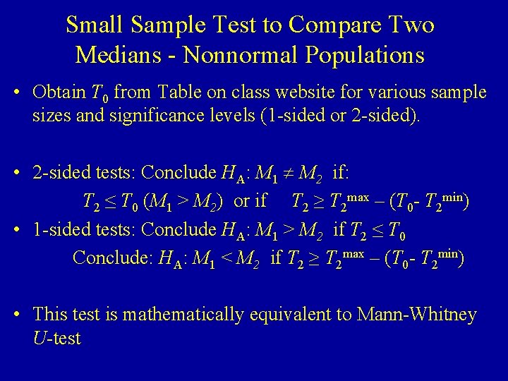
Small Sample Test to Compare Two Medians - Nonnormal Populations • Obtain T 0 from Table on class website for various sample sizes and significance levels (1 -sided or 2 -sided). • 2 -sided tests: Conclude HA: M 1 M 2 if: T 2 ≤ T 0 (M 1 > M 2) or if T 2 ≥ T 2 max – (T 0 - T 2 min) • 1 -sided tests: Conclude HA: M 1 > M 2 if T 2 ≤ T 0 Conclude: HA: M 1 < M 2 if T 2 ≥ T 2 max – (T 0 - T 2 min) • This test is mathematically equivalent to Mann-Whitney U-test

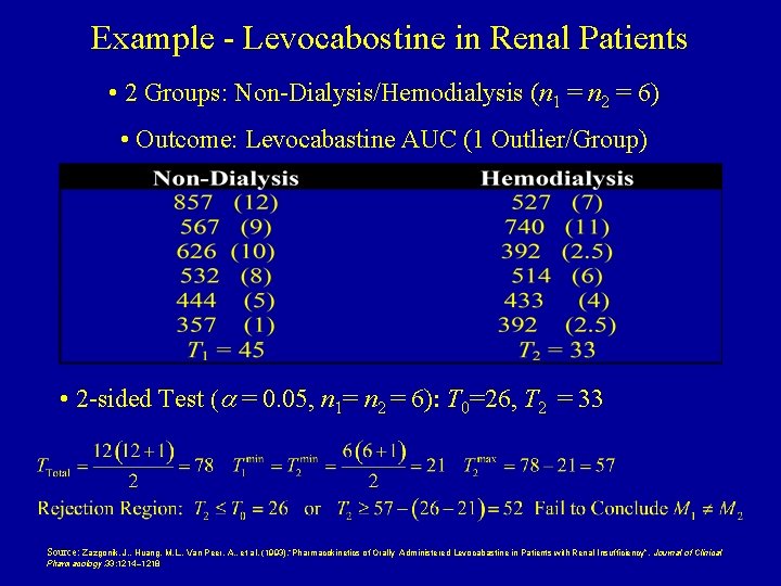
Example - Levocabostine in Renal Patients • 2 Groups: Non-Dialysis/Hemodialysis (n 1 = n 2 = 6) • Outcome: Levocabastine AUC (1 Outlier/Group) • 2 -sided Test (a = 0. 05, n 1= n 2 = 6): T 0=26, T 2 = 33 Source: Zazgonik, J. , Huang, M. L. , Van Peer, A. , et al. (1993), “Pharmacokinetics of Orally Pharmacology, 33: 1214– 1218 Administered Levocabastine in Patients with Renal Insufficiency”, Journal of Clinical

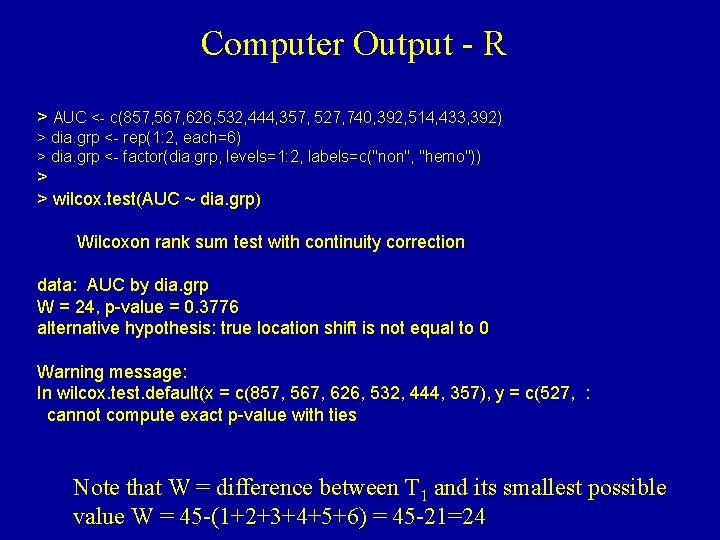
Computer Output - R > AUC <- c(857, 567, 626, 532, 444, 357, 527, 740, 392, 514, 433, 392) > dia. grp <- rep(1: 2, each=6) > dia. grp <- factor(dia. grp, levels=1: 2, labels=c("non", "hemo")) > > wilcox. test(AUC ~ dia. grp) Wilcoxon rank sum test with continuity correction data: AUC by dia. grp W = 24, p-value = 0. 3776 alternative hypothesis: true location shift is not equal to 0 Warning message: In wilcox. test. default(x = c(857, 567, 626, 532, 444, 357), y = c(527, : cannot compute exact p-value with ties Note that W = difference between T 1 and its smallest possible value W = 45 -(1+2+3+4+5+6) = 45 -21=24

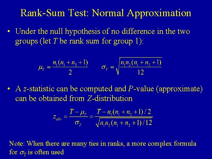
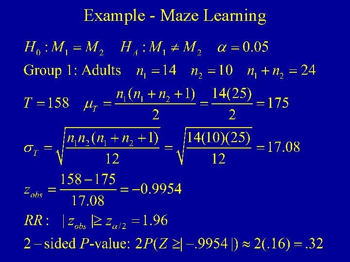
Rank-Sum Test: Normal Approximation • Under the null hypothesis of no difference in the two groups (let T be rank sum for group 1): • A z-statistic can be computed and P-value (approximate) can be obtained from Z-distribution Note: When there are many ties in ranks, a more complex formula for s. T is often used

Example - Maze Learning Adults = Group 1

Example - Maze Learning

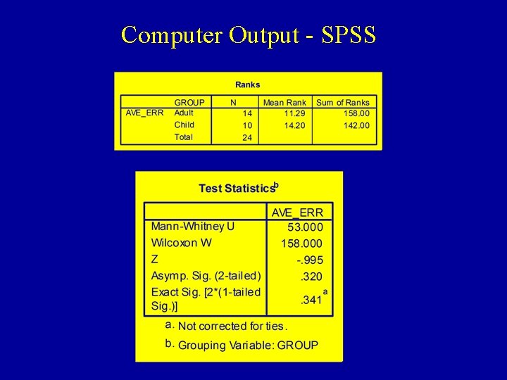
Computer Output - SPSS

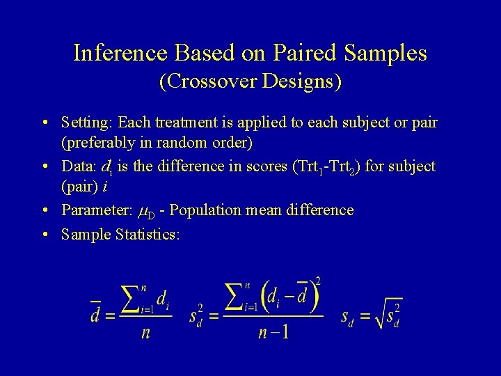
Inference Based on Paired Samples (Crossover Designs) • Setting: Each treatment is applied to each subject or pair (preferably in random order) • Data: di is the difference in scores (Trt 1 -Trt 2) for subject (pair) i • Parameter: m. D - Population mean difference • Sample Statistics:

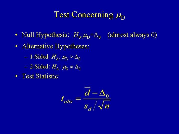
Test Concerning m. D • Null Hypothesis: H 0: m. D=D 0 (almost always 0) • Alternative Hypotheses: – 1 -Sided: HA: m. D > D 0 – 2 -Sided: HA: m. D D 0 • Test Statistic:

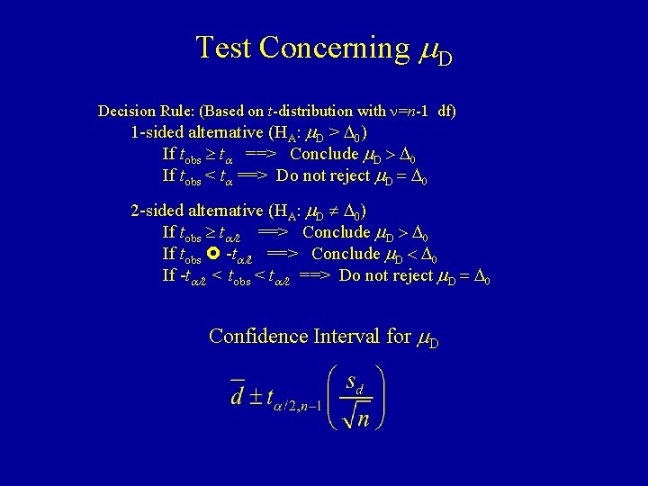
Test Concerning m. D Decision Rule: (Based on t-distribution with n=n-1 df) 1 -sided alternative (HA: m. D > D 0) If tobs ta ==> Conclude m. D > D 0 If tobs < ta ==> Do not reject m. D = D 0 2 -sided alternative (HA: m. D D 0) If tobs ta/2 ==> Conclude m. D > D 0 If tobs -ta/2 ==> Conclude m. D < D 0 If -ta/2 < tobs < ta/2 ==> Do not reject m. D = D 0 Confidence Interval for m. D

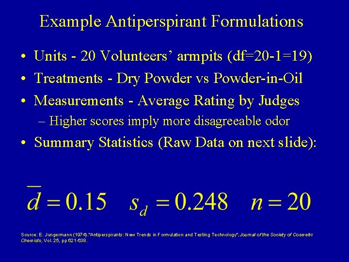
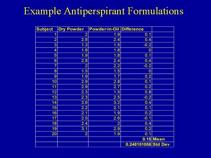
Example Antiperspirant Formulations • Units - 20 Volunteers’ armpits (df=20 -1=19) • Treatments - Dry Powder vs Powder-in-Oil • Measurements - Average Rating by Judges – Higher scores imply more disagreeable odor • Summary Statistics (Raw Data on next slide): Source: E. Jungermann (1974). "Antiperspirants: New Trends in Formulation and Testing Technology", Journal of the Society of Cosmetic Chemists, Vol. 25, pp 621 -638.

Example Antiperspirant Formulations

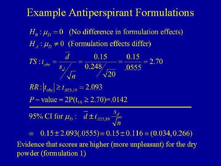
Example Antiperspirant Formulations Evidence that scores are higher (more unpleasant) for the dry powder (formulation 1)

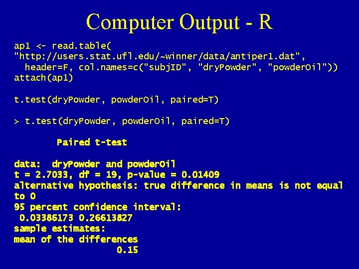
Computer Output - R ap 1 <- read. table( "http: //users. stat. ufl. edu/~winner/data/antiper 1. dat", header=F, col. names=c("subj. ID", "dry. Powder", "powder. Oil")) attach(ap 1) t. test(dry. Powder, powder. Oil, paired=T) > t. test(dry. Powder, powder. Oil, paired=T) Paired t-test data: dry. Powder and powder. Oil t = 2. 7033, df = 19, p-value = 0. 01409 alternative hypothesis: true difference in means is not equal to 0 95 percent confidence interval: 0. 03386173 0. 26613827 sample estimates: mean of the differences 0. 15

Small-Sample Test For Nonnormal Data • Paired Samples (Crossover Design) • Procedure (Wilcoxon Signed-Rank Test) – Compute Differences di (as in the paired t-test) and obtain their absolute values (ignoring 0 s). n= number of non-zero differences – Rank the observations by |di| (smallest=1), averaging ranks for ties – Compute T+ and T- , the rank sums for the positive and negative differences, respectively – 1 -sided tests: Conclude HA: M 1 > M 2 if T=T- T 0 – 2 -sided tests: Conclude HA: M 1 M 2 if T=min(T+ , T- ) T 0 – Values of T 0 are given in Table on website for various sample sizes and commonly used a levels for 1 - and 2 -sided tests. P-values printed by statistical software packages.

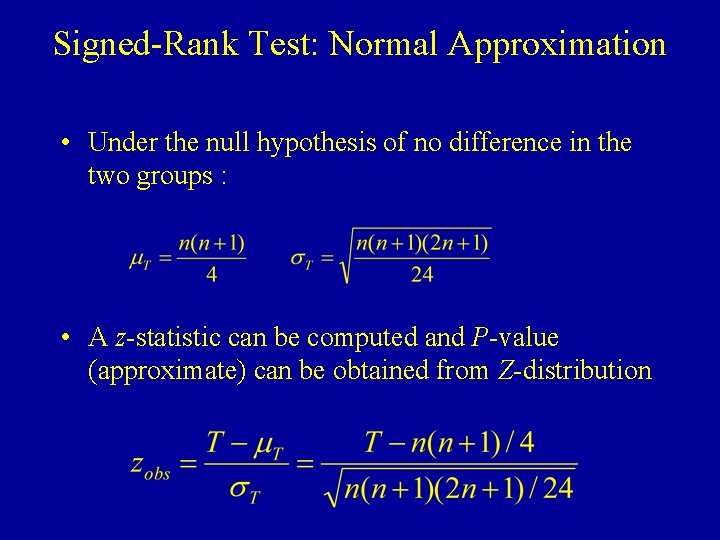
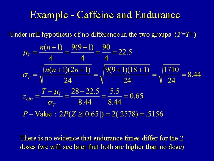
Signed-Rank Test: Normal Approximation • Under the null hypothesis of no difference in the two groups : • A z-statistic can be computed and P-value (approximate) can be obtained from Z-distribution

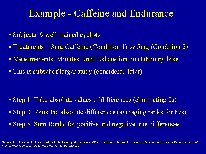
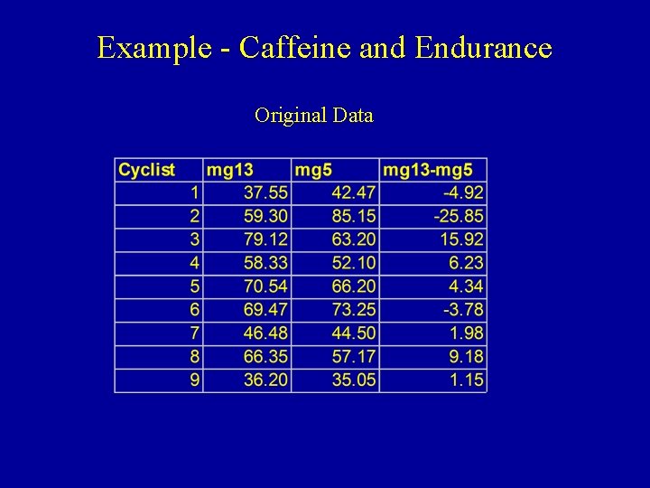
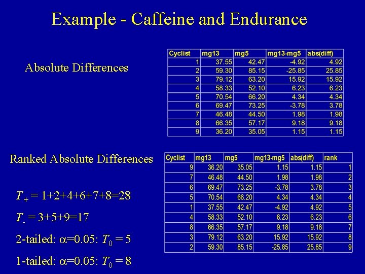
Example - Caffeine and Endurance • Subjects: 9 well-trained cyclists • Treatments: 13 mg Caffeine (Condition 1) vs 5 mg (Condition 2) • Measurements: Minutes Until Exhaustion on stationary bike • This is subset of larger study (considered later) • Step 1: Take absolute values of differences (eliminating 0 s) • Step 2: Rank the absolute differences (averaging ranks for ties) • Step 3: Sum Ranks for positive and negative true differences Source: W. J. Pasman, M. A. van Baak, A. E. Jeukendrup, A. de Haan (1995). "The Effect of Different Dosages of Caffeine on Endurance Performance Time", International Journal of Sports Medicine, Vol. 16, pp. 225 -230.

Example - Caffeine and Endurance Original Data

Example - Caffeine and Endurance Absolute Differences Ranked Absolute Differences T+ = 1+2+4+6+7+8=28 T- = 3+5+9=17 2 -tailed: a=0. 05: T 0 = 5 1 -tailed: a=0. 05: T 0 = 8

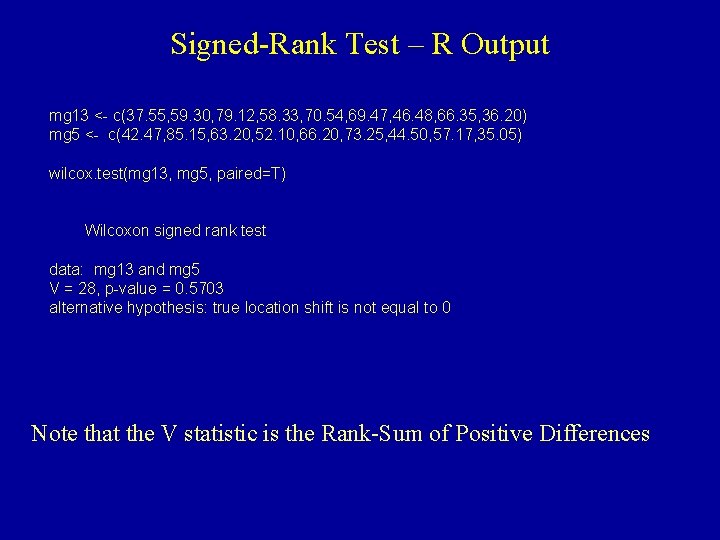
Signed-Rank Test – R Output mg 13 <- c(37. 55, 59. 30, 79. 12, 58. 33, 70. 54, 69. 47, 46. 48, 66. 35, 36. 20) mg 5 <- c(42. 47, 85. 15, 63. 20, 52. 10, 66. 20, 73. 25, 44. 50, 57. 17, 35. 05) wilcox. test(mg 13, mg 5, paired=T) Wilcoxon signed rank test data: mg 13 and mg 5 V = 28, p-value = 0. 5703 alternative hypothesis: true location shift is not equal to 0 Note that the V statistic is the Rank-Sum of Positive Differences

Example - Caffeine and Endurance Under null hypothesis of no difference in the two groups (T=T+): There is no evidence that endurance times differ for the 2 doses (we will see later that both are higher than no dose)

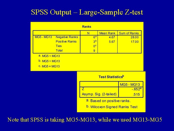
SPSS Output – Large-Sample Z-test Note that SPSS is taking MG 5 -MG 13, while we used MG 13 -MG 5

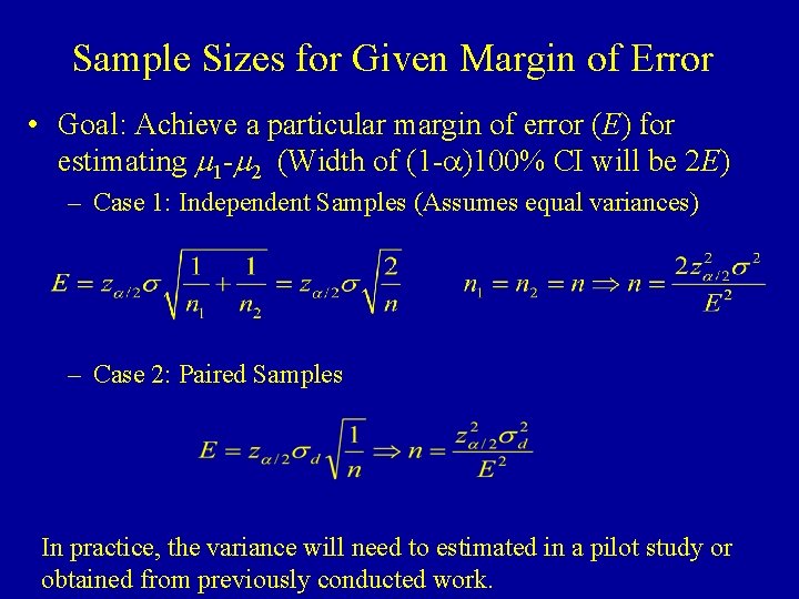
Sample Sizes for Given Margin of Error • Goal: Achieve a particular margin of error (E) for estimating m 1 -m 2 (Width of (1 -a)100% CI will be 2 E) – Case 1: Independent Samples (Assumes equal variances) – Case 2: Paired Samples In practice, the variance will need to estimated in a pilot study or obtained from previously conducted work.

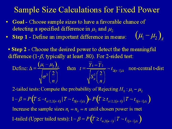
Sample Size Calculations for Fixed Power • Goal - Choose sample sizes to have a favorable chance of detecting a specified difference in m 1 and m 2 • Step 1 - Define an important difference in means: • Step 2 - Choose the desired power to detect the meaningful difference (1 -b, typically at least. 80). For 2 -sided test:

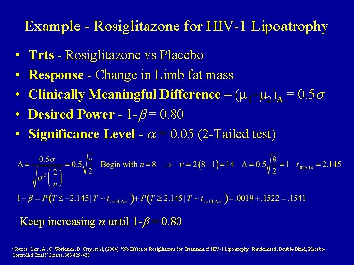
Example - Rosiglitazone for HIV-1 Lipoatrophy • • • Trts - Rosiglitazone vs Placebo Response - Change in Limb fat mass Clinically Meaningful Difference – (m 1 -m 2)A = 0. 5 s Desired Power - 1 -b = 0. 80 Significance Level - a = 0. 05 (2 -Tailed test) Keep increasing n until 1 -b = 0. 80 • Source: Carr, A. , C. Workman, D. Crey, et al, (2004). “No Effect of Rosiglitazone for Treatment of HIV-1 Lipoatrophy: Randomised, Double-Blind, Placebo. Controlled Trial, ” Lancet, 363: 429 -438

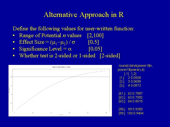
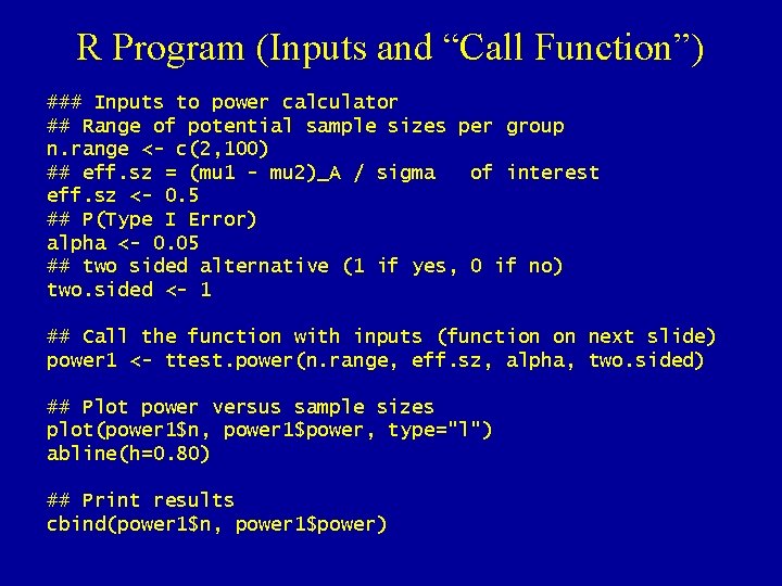
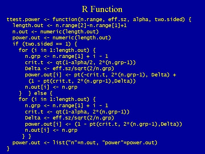
Alternative Approach in R Define the following values for user-written function: • Range of Potential n values [2, 100] • Effect Size = (m 1 -m 2) / s [0. 5] • Significance Level = a [0. 05] • Whether test is 2 -sided or 1 -sided [2 -sided] round(cbind(power 1$n, power 1$power), 4) [, 1] [, 2] [1, ] 2 0. 0508 [2, ] 3 0. 0698 [3, ] 4 0. 0872 … [61, ] 62 0. 7887 [62, ] 63 0. 7952 [63, ] 64 0. 8015 … [98, ] 99 0. 9383 [99, ] 100 0. 9404

R Program (Inputs and “Call Function”) ### Inputs to power calculator ## Range of potential sample sizes per group n. range <- c(2, 100) ## eff. sz = (mu 1 - mu 2)_A / sigma of interest eff. sz <- 0. 5 ## P(Type I Error) alpha <- 0. 05 ## two sided alternative (1 if yes, 0 if no) two. sided <- 1 ## Call the function with inputs (function on next slide) power 1 <- ttest. power(n. range, eff. sz, alpha, two. sided) ## Plot power versus sample sizes plot(power 1$n, power 1$power, type="l") abline(h=0. 80) ## Print results cbind(power 1$n, power 1$power)

R Function ttest. power <- function(n. range, eff. sz, alpha, two. sided) { length. out <- n. range[2]-n. range[1]+1 n. out <- numeric(length. out) power. out <- numeric(length. out) if (two. sided == 1) { for (i in 1: length. out) { n. grp <- n. range[1] + i - 1 crit. t <- qt(1 -alpha/2, 2*(n. grp-1)) Delta <- eff. sz/sqrt(2/n. grp) power. out[i] <- pt(-crit. t, 2*(n. grp-1), Delta) + (1 - pt(crit. t, 2*(n. grp-1), Delta)) n. out[i] <- n. grp } } else { for (i in 1: length. out) { n. grp <- n. range[1] + i - 1 crit. t <- qt(1 -alpha, 2*(n. grp-1)) Delta <- eff. sz/sqrt(2/n. grp) power. out[i] <- (1 - pt(crit. t, 2*(n. grp-1), Delta)) n. out[i] <- n. grp } } power. out <- list("n"=n. out, "power"=power. out) }