3 1 ECONOMICS ELEVENTH EDITION LIPSEY CHRYSTAL Chapter

3 - 1 ECONOMICS ELEVENTH EDITION LIPSEY & CHRYSTAL Chapter 3 DEMAND, SUPPLY, AND PRICE Slides by Alex Stojanovic

3 - 2 Learning Outcomes • The participants in markets and what motivates them • The main factors that influence how much of a product consumers wish to buy • The main influences on how much producers wish to sell • How consumers and producers interact to determine the market price • While demand supply forces are present in all markets, many different institutional structures also affect market outcomes

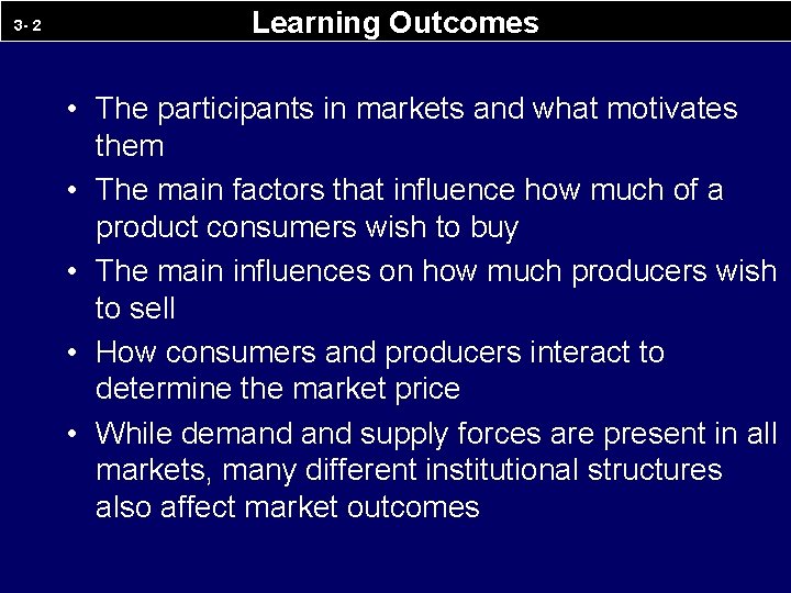
DEMAND 3 - 3 Alice’s Demand Schedule Price [£ per dozen] Quantity demanded [dozen per month] a b c d e f 0. 50 1. 00 1. 50 2. 00 2. 50 3. 00 7. 0 5. 0 3. 5 2. 5 1. 0 Alice’s Demand Curve Price of eggs [£ per dozen] Reference Letter 3. 00 f e 2. 50 d 2. 00 c 1. 50 b 1. 00 a 0. 50 1 2 3 4 5 6 7 Quantity of Eggs [dozen per month]

3 - 4 Alice’s demand schedule for eggs · The table shows the quantity of eggs that Alice will demand at each selected price, other things being equal. · For example, at a price of £ 1. 00, Alice demands 5 dozen eggs per month. · The data is plotted in Figure ‘Alice’s demand curve’.

3 - 5 Alice’s demand curve · Each point on the figure relates to a row on Table Demand Schedule. · For example, when price is £ 3. 00, 1 dozen are brought per month (point f ). · When the price is £ 0. 50, 7 dozen are brought (point a). · The resulting curve relates the price of a commodity to the amount that Alice wishes to purchase.

The Relation Between Individual and Market Demand Curves 3. 00 2. 00 1. 00 3. 00 2 Price of eggs [£ per dozen] [i]. William 4 6 8 Quantity of Eggs [dozen per month] 3. 00 2. 00 1. 00 2 4 6 8 10 12 Quantity of Eggs [dozen per month] 1. 00 [ii]. Sarah Price of eggs [£ per dozen] 3 - 6 [iii]. Total Demand William & Sarah 2 4 Quantity of Eggs [dozen per month] 6 8 14

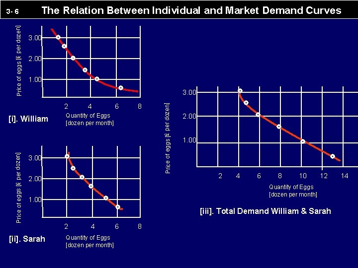
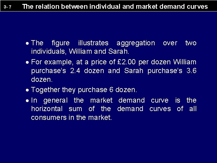
3 - 7 The relation between individual and market demand curves · The figure illustrates aggregation over two individuals, William and Sarah. · For example, at a price of £ 2. 00 per dozen William purchase’s 2. 4 dozen and Sarah purchase’s 3. 6 dozen. · Together they purchase 6 dozen. · In general the market demand curve is the horizontal sum of the demand curves of all consumers in the market.

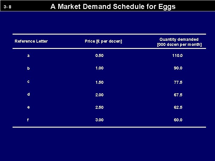
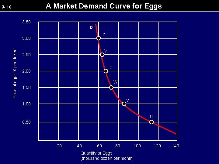
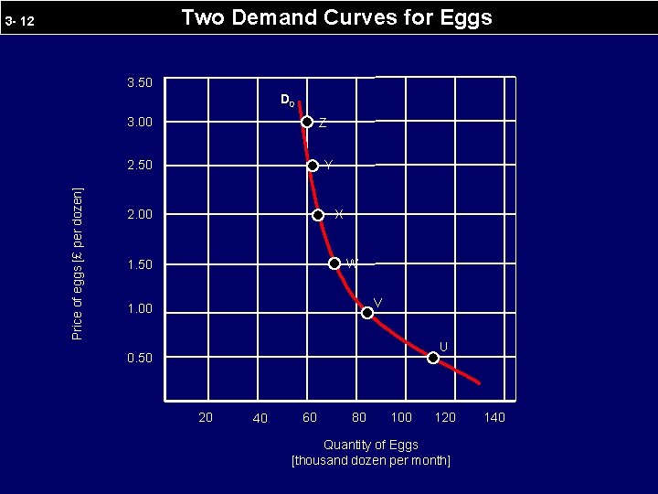
A Market Demand Schedule for Eggs 3 - 8 Reference Letter Price [£ per dozen] Quantity demanded [000 dozen per month] a 0. 50 110. 0 b 1. 00 90. 0 c 1. 50 77. 5 d 2. 00 67. 5 e 2. 50 62. 5 f 3. 00 60. 0

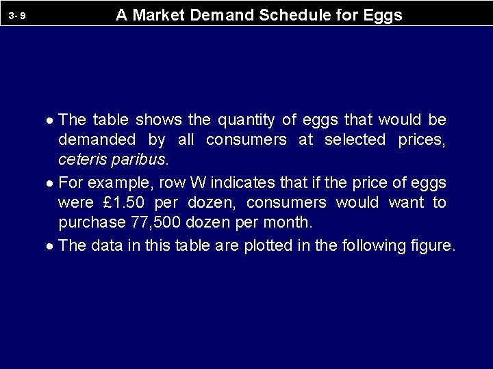
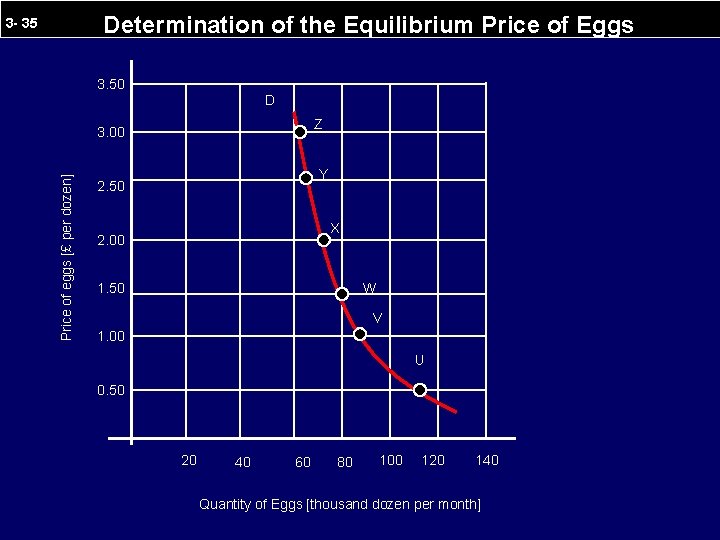
3 - 9 A Market Demand Schedule for Eggs · The table shows the quantity of eggs that would be demanded by all consumers at selected prices, ceteris paribus. · For example, row W indicates that if the price of eggs were £ 1. 50 per dozen, consumers would want to purchase 77, 500 dozen per month. · The data in this table are plotted in the following figure.

A Market Demand Curve for Eggs 3 - 10 3. 50 D Z Price of eggs [£ per dozen] 3. 00 Y 2. 50 X 2. 00 W 1. 50 V 1. 00 U 0. 50 20 40 60 80 100 Quantity of Eggs [thousand dozen per month] 120 140

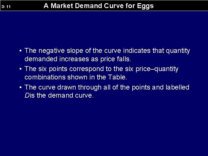
3 - 11 A Market Demand Curve for Eggs • The negative slope of the curve indicates that quantity demanded increases as price falls. • The six points correspond to the six price–quantity combinations shown in the Table. • The curve drawn through all of the points and labelled Dis the demand curve.

Two Demand Curves for Eggs 3 - 12 3. 50 D 0 3. 00 Z Price of eggs [£ per dozen] 2. 50 Y 2. 00 X W 1. 50 V 1. 00 U 0. 50 20 40 60 80 100 120 Quantity of Eggs [thousand dozen per month] 140

Two Demand Curves for Eggs 3 - 13 3. 50 D 1 D 0 3. 00 2. 50 Price of eggs [£ per dozen] Z’ Z Y 2. 00 Y’ X X’ W 1. 50 W’ V’ V 1. 00 U 0. 50 20 40 60 80 100 120 Quantity of Eggs [thousand dozen per month] U’ 140

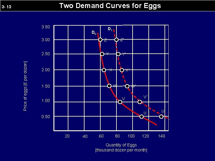
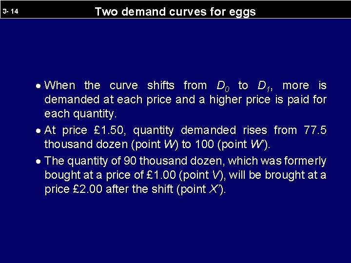
3 - 14 Two demand curves for eggs · When the curve shifts from D 0 to D 1, more is demanded at each price and a higher price is paid for each quantity. · At price £ 1. 50, quantity demanded rises from 77. 5 thousand dozen (point W) to 100 (point W’). · The quantity of 90 thousand dozen, which was formerly bought at a price of £ 1. 00 (point V), will be brought at a price £ 2. 00 after the shift (point X’).

Shifts in the Demand Curve 3 - 15 Price D 0 0 Quantity

Shifts in the Demand Curve 3 - 16 D 1 Price D 0 0 Quantity

Shifts in the Demand Curve 3 - 17 D 1 D 0 Price D 2 0 Quantity

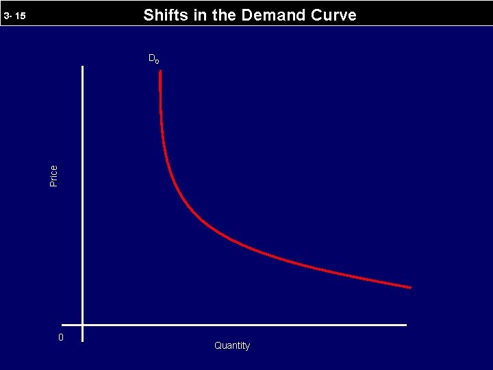
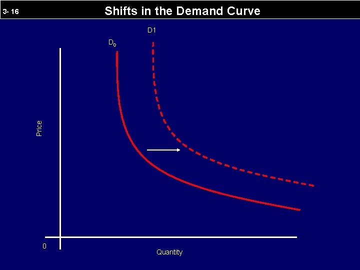
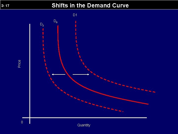
3 - 18 Shifts in the demand curve · When the demand curve shifts from D 0 to D 1, more is demanded at each price. · Such and increase in demand can be caused by: · A rise in the price of a substitute · A fall in the price of a complement · A rise in income · A redistribution of income towards those who favour the commodity · A change in tastes that favours the commodity

3 - 19 Shifts in the demand curve · When the demand curve shifts from D 0 to D 2, less is demanded at each price. · Such a decrease in demand can be caused by: · a fall in the price of a substitute · a rise in the price of a complement, a fall in income · a redistribution of income away from groups that favour the commodity · a change in tastes that disfavours the commodity

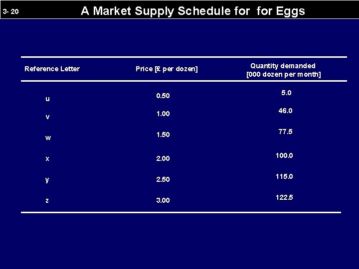
A Market Supply Schedule for Eggs 3 - 20 Reference Letter Price [£ per dozen] Quantity demanded [000 dozen per month] u 0. 50 5. 0 v 1. 00 46. 0 w 1. 50 77. 5 x 2. 00 100. 0 y 2. 50 115. 0 z 3. 00 122. 5

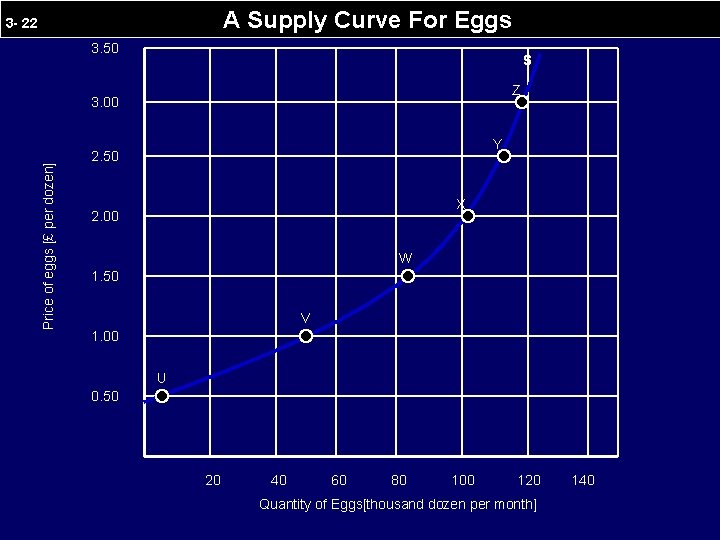
3 - 21 A market supply schedule for eggs · The table shows the quantities that producers wish to sell at various prices, ceteris paribus. · For example, row y indicates that if the price were £ 2. 50, producers would wish to sell 115, 000 dozen eggs per month. · The data in this table are plotted in the following figure.

A Supply Curve For Eggs 3 - 22 3. 50 S Z Price of eggs [£ per dozen] 3. 00 Y 2. 50 X 2. 00 W 1. 50 V 1. 00 U 0. 50 20 40 60 80 100 120 Quantity of Eggs[thousand dozen per month] 140

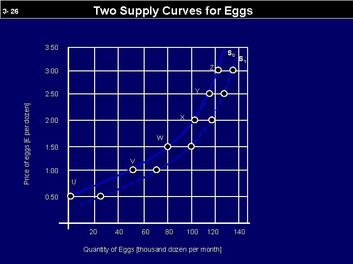
3 - 23 A supply curve for eggs · The six points correspond to the price-quantity combinations shown in Table ‘A Market Supply Schedule for Eggs’. · The curve drawn through these points, labeled S, is the supply curve showing the quantity of eggs that will be supplied at each price of eggs. · The supply curve’s positive slope indicates that quantity supplied increases as price increases.

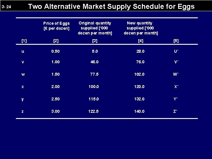
Two Alternative Market Supply Schedule for Eggs 3 - 24 Price of Eggs [£ per dozen] Original quantity supplied [‘ 000 dozen per month] New quantity supplied [‘ 000 dozen per month] [2] [3] [4] [5] u 0. 50 5. 0 28. 0 U’ v 1. 00 46. 0 76. 0 V’ w 1. 50 77. 5 102. 0 W’ x 2. 00 100. 0 120. 0 X’ y 2. 50 115. 0 132. 0 Y’ z 3. 00 122. 5 140. 0 Z’ [1]

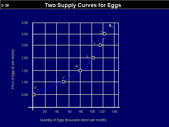
Two Supply Curves for Eggs 3 - 25 3. 50 S 0 Z 3. 00 Y Price of eggs [£ per dozen] 2. 50 X 2. 00 W 1. 50 V 1. 00 U 0. 50 20 40 60 80 100 120 Quantity of Eggs [thousand dozen per month] 140

Two Supply Curves for Eggs 3 - 26 3. 50 S 0 Z 3. 00 Y 2. 50 Price of eggs [£ per dozen] S 1 X 2. 00 W 1. 50 V 1. 00 U 0. 50 20 40 60 80 100 120 Quantity of Eggs [thousand dozen per month] 140

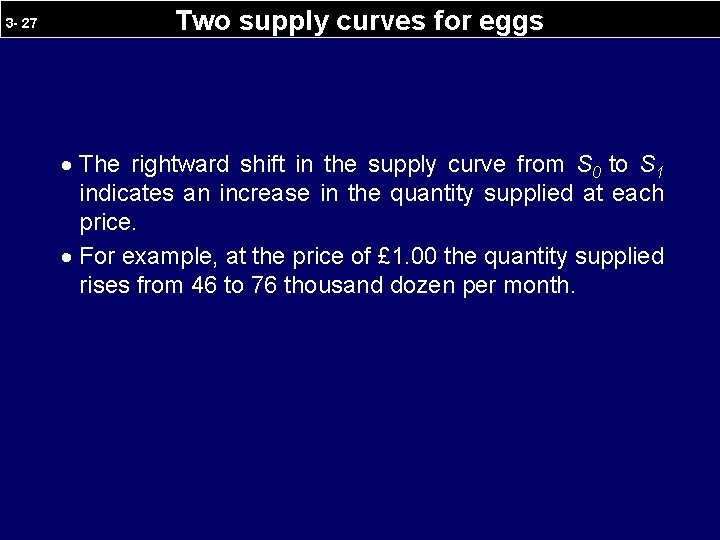
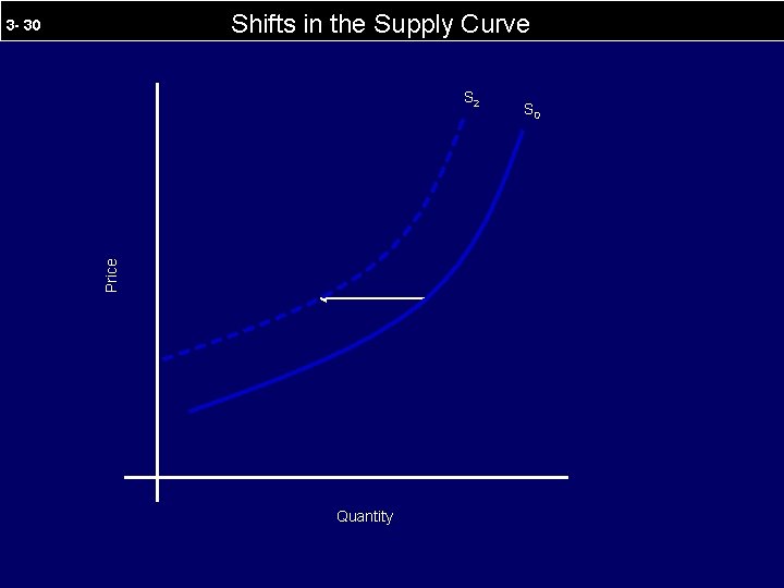
3 - 27 Two supply curves for eggs · The rightward shift in the supply curve from S 0 to S 1 indicates an increase in the quantity supplied at each price. · For example, at the price of £ 1. 00 the quantity supplied rises from 46 to 76 thousand dozen per month.

Shifts in the Supply Curve 3 - 28 Price S 0 Quantity

Shifts in the Supply Curve 3 - 29 Price S 0 Quantity S 1

Shifts in the Supply Curve 3 - 30 Price S 2 Quantity S 0

Shifts in the Supply Curve 3 - 31 Price S 2 Quantity S 0 S 1

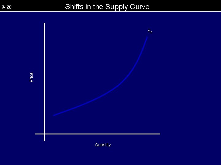
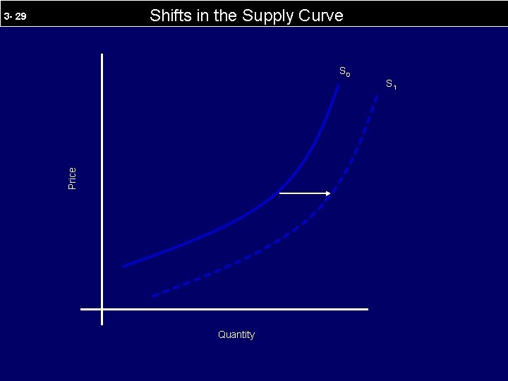
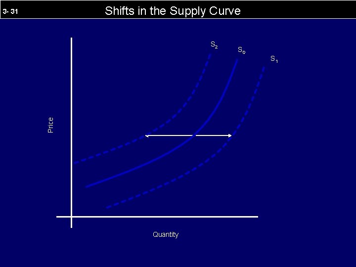
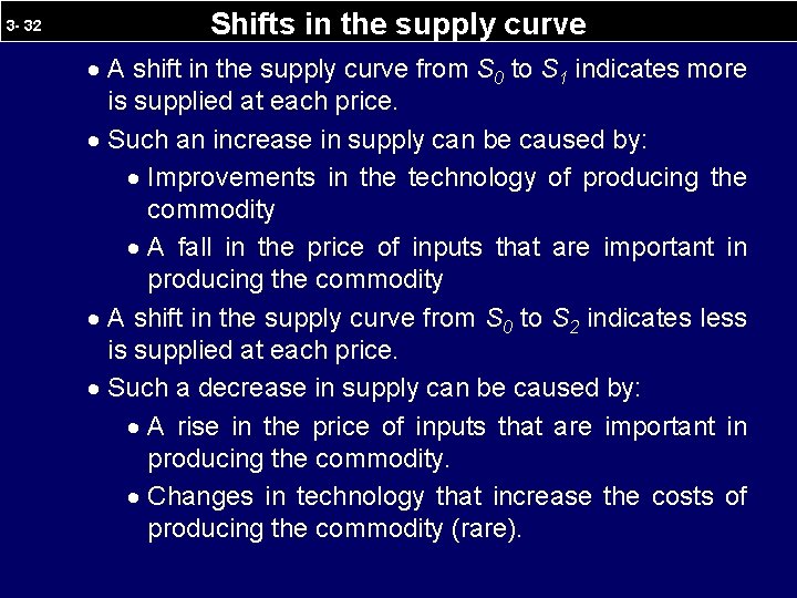
3 - 32 Shifts in the supply curve · A shift in the supply curve from S 0 to S 1 indicates more is supplied at each price. · Such an increase in supply can be caused by: · Improvements in the technology of producing the commodity · A fall in the price of inputs that are important in producing the commodity · A shift in the supply curve from S 0 to S 2 indicates less is supplied at each price. · Such a decrease in supply can be caused by: · A rise in the price of inputs that are important in producing the commodity. · Changes in technology that increase the costs of producing the commodity (rare).

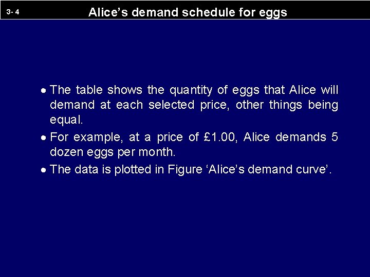
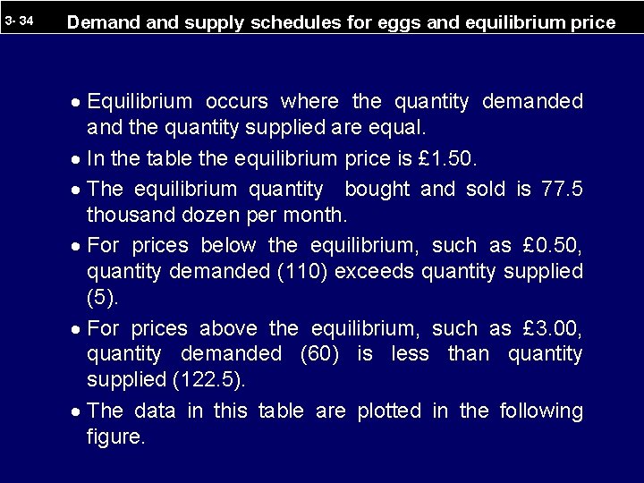
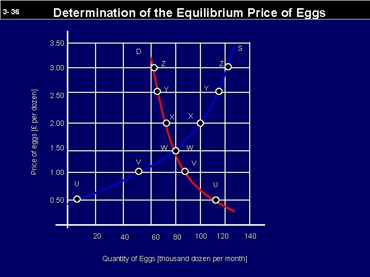
3 - 33 Demand Supply Schedules for Eggs and Equilibrium Price [£ per dozen] Quantity demanded [‘ 000 dozen per month] Quantity supplied [‘ 000 dozen per month] Excess Demand [quantity demanded minus quantity supplied] [‘ 000 dozen per month] 0. 50 110. 0 5. 0 105. 0 1. 00 90. 0 46. 0 44. 0 1. 50 77. 5 0. 0 2. 00 67. 5 100. 0 -32. 50 62. 5 115. 0 -52. 5 3. 00 60. 0 122. 5 -62. 5

3 - 34 Demand supply schedules for eggs and equilibrium price · Equilibrium occurs where the quantity demanded and the quantity supplied are equal. · In the table the equilibrium price is £ 1. 50. · The equilibrium quantity bought and sold is 77. 5 thousand dozen per month. · For prices below the equilibrium, such as £ 0. 50, quantity demanded (110) exceeds quantity supplied (5). · For prices above the equilibrium, such as £ 3. 00, quantity demanded (60) is less than quantity supplied (122. 5). · The data in this table are plotted in the following figure.

Determination of the Equilibrium Price of Eggs 3 - 35 3. 50 D Z Price of eggs [£ per dozen] 3. 00 Y 2. 50 X 2. 00 1. 50 W V 1. 00 U 0. 50 20 40 60 80 100 120 140 Quantity of Eggs [thousand dozen per month]

Determination of the Equilibrium Price of Eggs 3 - 36 3. 50 S D Z Price of eggs [£ per dozen] 3. 00 Z Y Y 2. 50 X 2. 00 1. 50 W X W V V 1. 00 U U 0. 50 20 40 60 80 100 120 140 Quantity of Eggs [thousand dozen per month]

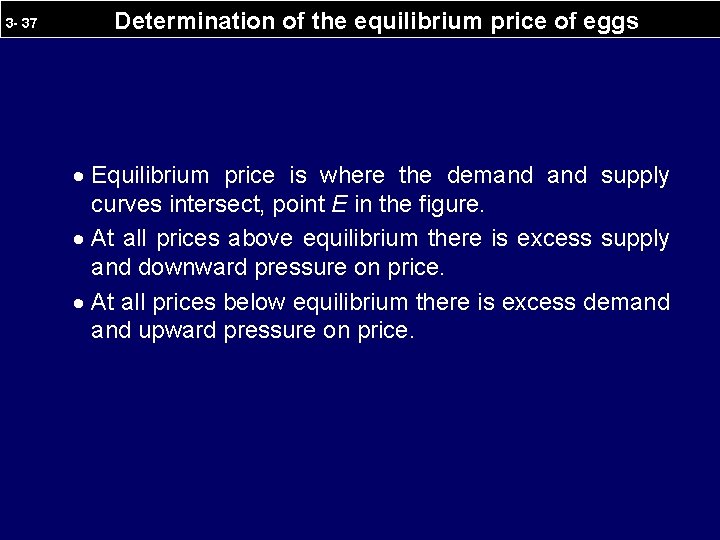
3 - 37 Determination of the equilibrium price of eggs · Equilibrium price is where the demand supply curves intersect, point E in the figure. · At all prices above equilibrium there is excess supply and downward pressure on price. · At all prices below equilibrium there is excess demand upward pressure on price.

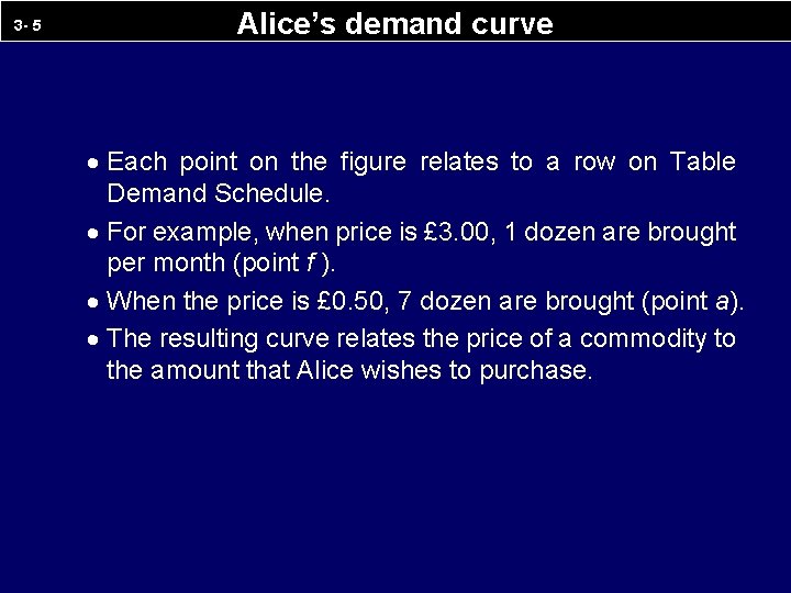
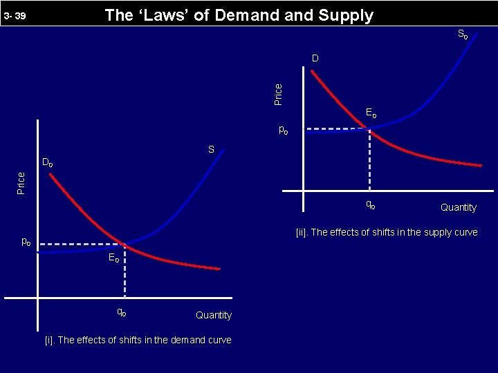
3 - 38 The ‘Laws’ of Demand Supply Price D Price S Quantity [ii]. The effects of shifts in the supply curve Quantity [i]. The effects of shifts in the demand curve

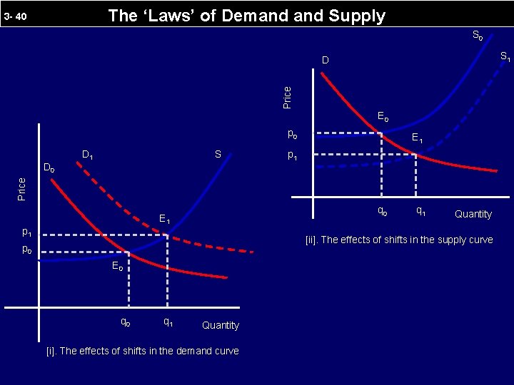
The ‘Laws’ of Demand Supply 3 - 39 S 0 Price D E 0 p 0 S Price D 0 q 0 Quantity [ii]. The effects of shifts in the supply curve p 0 E 0 q 0 Quantity [i]. The effects of shifts in the demand curve

The ‘Laws’ of Demand Supply 3 - 40 S 1 Price D E 0 p 0 S p 1 Price D 0 D 1 E 1 q 0 E 1 p 1 q 1 Quantity [ii]. The effects of shifts in the supply curve p 0 E 0 q 1 Quantity [i]. The effects of shifts in the demand curve

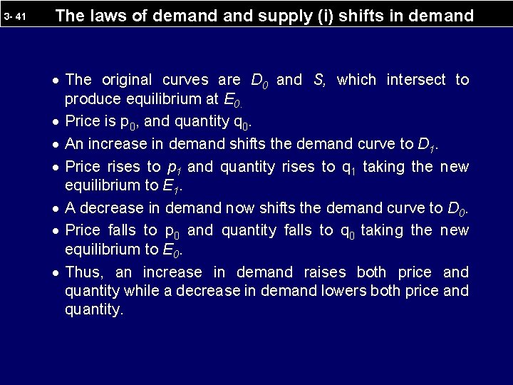
3 - 41 The laws of demand supply (i) shifts in demand · The original curves are D 0 and S, which intersect to produce equilibrium at E 0. · Price is p 0, and quantity q 0. · An increase in demand shifts the demand curve to D 1. · Price rises to p 1 and quantity rises to q 1 taking the new equilibrium to E 1. · A decrease in demand now shifts the demand curve to D 0. · Price falls to p 0 and quantity falls to q 0 taking the new equilibrium to E 0. · Thus, an increase in demand raises both price and quantity while a decrease in demand lowers both price and quantity.

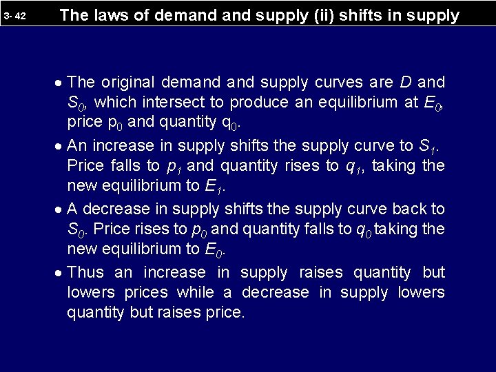
3 - 42 The laws of demand supply (ii) shifts in supply · The original demand supply curves are D and S 0, which intersect to produce an equilibrium at E 0, price p 0 and quantity q 0. · An increase in supply shifts the supply curve to S 1. Price falls to p 1 and quantity rises to q 1, taking the new equilibrium to E 1. · A decrease in supply shifts the supply curve back to S 0. Price rises to p 0 and quantity falls to q 0 taking the new equilibrium to E 0. · Thus an increase in supply raises quantity but lowers prices while a decrease in supply lowers quantity but raises price.

3 - 43 CHAPTER 3: DEMAND, SUPPLY AND PRICE • The decision-taking units in economic theory are called agents. • They are [a] individuals, for the demand in goods markets and for supply in factor markets; [b] firms, for supply in goods markets and demand in factor markets; and [c] governments, for supply of some goods and for regulation and control of the private sector [see Chapter 5]. • Given the resources at their command, each individual is assumed to maximize his or her satisfaction, and each firm is assumed to maximize its profit.

3 - 44 CHAPTER 3: DEMAND, SUPPLY AND PRICE Demand • An individual consumer’s demand curve shows the relation between the price of a product and the quantity of that product the customer wishes to purchase period of time. • It is drawn on the assumption that all other prices, income, and tastes remain constant. • Its negative slope indicates that the lower the price of the product, the more the consumer wishes to purchase. • The market demand curve is the horizontal sum of all the individual consumers.

CHAPTER 3: DEMAND, SUPPLY AND PRICE 3 - 45 • The demand curve for a normal good shifts to the right when the price of a substitute rises, when the price of a complement falls, when total income rises, when the distribution of income changes in favour of those with large demands for the product, and when tastes change in favour of the product It shifts to the left with the opposite changes. • A movement along a demand curve indicates a change in quantity demanded in response to a change in the product’s own price; a shift in a demand curve indicates a change in the quantity demanded at each price in response to a change in one of the conditions held constant along a demand curve. •

3 - 46 CHAPTER 3: DEMAND, SUPPLY AND PRICE Supply • The supply curve for a product shows the relationship between its price and the quantity that producers wish to produce and offer for sale period of time. • It is drawn on the assumption that all other forces that influence quantity supplied remain constant, and its positive slope indicates that the higher price, the more producers wish to sell.

3 - 47 CHAPTER 3: DEMAND, SUPPLY AND PRICE The Determination of Price • At the equilibrium price the quantity demanded equals the quantity supplied. • Graphically, equilibrium occurs where the demand supply curves intersect. • At any price below equilibrium there will be excess demand price will tend to rise; at any price above equilibrium there will be excess supply and price will tend to fall. • A rise in demand raises both equilibrium price and quantity; a fall in demand lowers both. • A rise in supply raises equilibrium quantity but lowers equilibrium price; a fall in supply lowers equilibrium quantity but raises equilibrium price. • These are those so-called ‘laws’ of supply and demand.

3 - 48 CHAPTER 3: DEMAND, SUPPLY AND PRICE • Price theory is most simply developed in the context of a constant price level. • Price changes discussed in theory are changes relative to the average level of all prices. • In an inflationary period, a rise in the relative price of one product means that its price rises by more than the rise in the general price level; a fall in its relative price means that its price rises by less than the rise in the general price level.

3 - 49 CHAPTER 3: DEMAND, SUPPLY AND PRICE Individual markets, sectors, and the economy • Markets are partially separated from each other because different products are sold in each, and because of barriers to the movement of products among such markets as transport costs [a natural barrier] and tariffs [ a policy-induced barrier]. • For various types of study, data for individual markets are aggregated into sectors. • Examples are primary, secondary, and tertiary, a distinction on the types of goods produced; private and public, a distinction depending on whether or not the costs of production are recovered by selling products to their users.