7 1 ECONOMICS ELEVENTH EDITION LIPSEY CHRYSTAL Chapter

7 - 1 ECONOMICS ELEVENTH EDITION LIPSEY & CHRYSTAL Chapter 7 PERFECT COMPETITION Slides by Alex Stojanovic

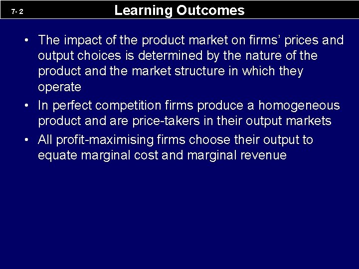
7 - 2 Learning Outcomes • The impact of the product market on firms’ prices and output choices is determined by the nature of the product and the market structure in which they operate • In perfect competition firms produce a homogeneous product and are price-takers in their output markets • All profit-maximising firms choose their output to equate marginal cost and marginal revenue

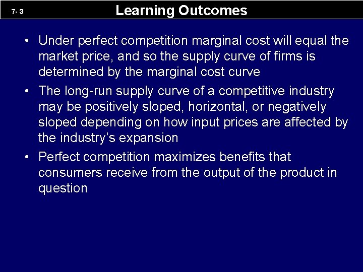
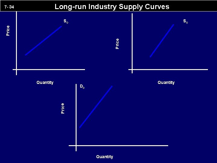
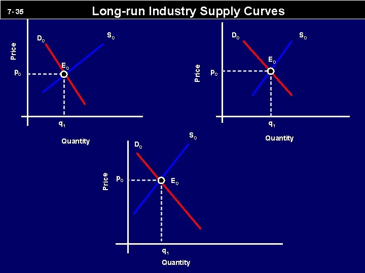
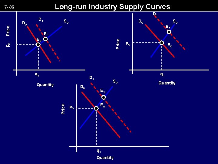
7 - 3 Learning Outcomes • Under perfect competition marginal cost will equal the market price, and so the supply curve of firms is determined by the marginal cost curve • The long-run supply curve of a competitive industry may be positively sloped, horizontal, or negatively sloped depending on how input prices are affected by the industry’s expansion • Perfect competition maximizes benefits that consumers receive from the output of the product in question

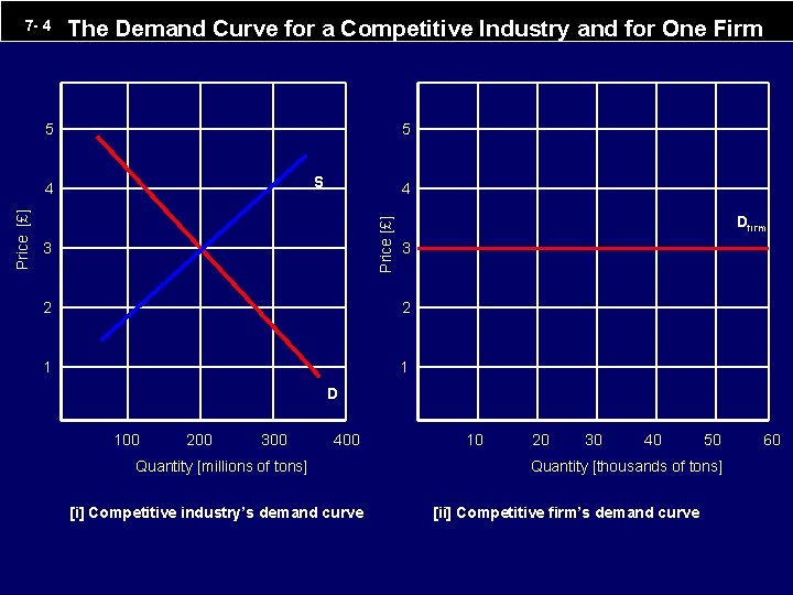
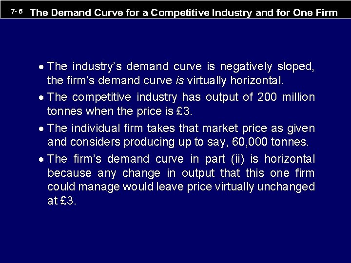
7 - 4 The Demand Curve for a Competitive Industry and for One Firm 5 5 S 4 Price [£] 4 3 Dfirm 3 2 2 1 1 D 100 200 300 400 Quantity [millions of tons] [i] Competitive industry’s demand curve 10 20 30 40 50 Quantity [thousands of tons] [ii] Competitive firm’s demand curve 60

7 - 5 The Demand Curve for a Competitive Industry and for One Firm · The industry’s demand curve is negatively sloped, the firm’s demand curve is virtually horizontal. · The competitive industry has output of 200 million tonnes when the price is £ 3. · The individual firm takes that market price as given and considers producing up to say, 60, 000 tonnes. · The firm’s demand curve in part (ii) is horizontal because any change in output that this one firm could manage would leave price virtually unchanged at £ 3.

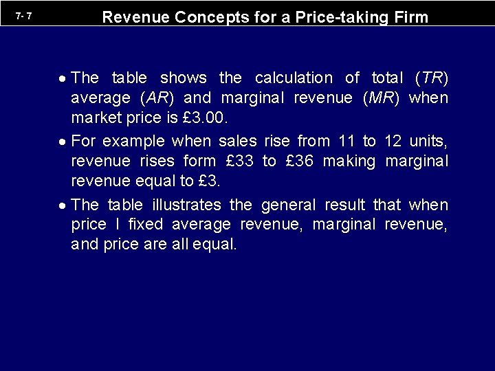
Revenue Concepts for a Price-taking Firm 7 - 6 Quantity sold [units] Price [q] [p] 10 £ 3, 00 £ 30, 00 £ 3, 00 11 3, 00 12 3, 00 36, 00 3, 00 13 3, 00 39, 00 3, 00 TR = p*q AR = TR/q MR = TR/ q £ 3, 00

7 - 7 Revenue Concepts for a Price-taking Firm · The table shows the calculation of total (TR) average (AR) and marginal revenue (MR) when market price is £ 3. 00. · For example when sales rise from 11 to 12 units, revenue rises form £ 33 to £ 36 making marginal revenue equal to £ 3. · The table illustrates the general result that when price I fixed average revenue, marginal revenue, and price are all equal.

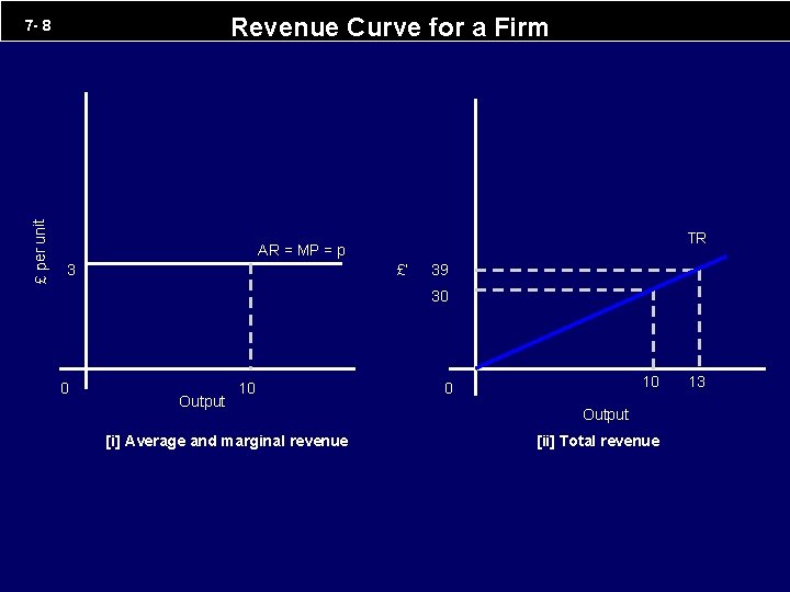
Revenue Curve for a Firm £ per unit 7 - 8 TR AR = MP = p 3 £’ 39 30 0 Output 10 [i] Average and marginal revenue 10 0 Output [ii] Total revenue 13

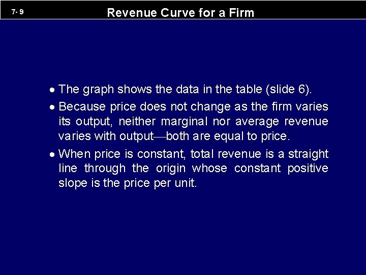
7 - 9 Revenue Curve for a Firm · The graph shows the data in the table (slide 6). · Because price does not change as the firm varies its output, neither marginal nor average revenue varies with output both are equal to price. · When price is constant, total revenue is a straight line through the origin whose constant positive slope is the price per unit.

The Short-run Equilibrium of a Firm in Perfect Competition 7 - 10 £ per unit AVC Output

The Short-run Equilibrium of a Firm in Perfect Competition 7 - 11 £ per unit MC AVC Output

The Short-run Equilibrium of a Firm in Perfect Competition 7 - 12 £ per unit MC AVC E p=MR=AR q 2 q. E Output q 1

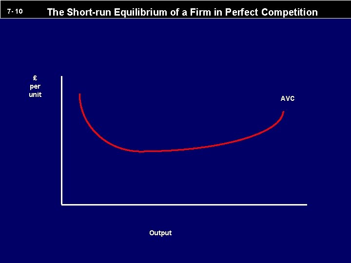
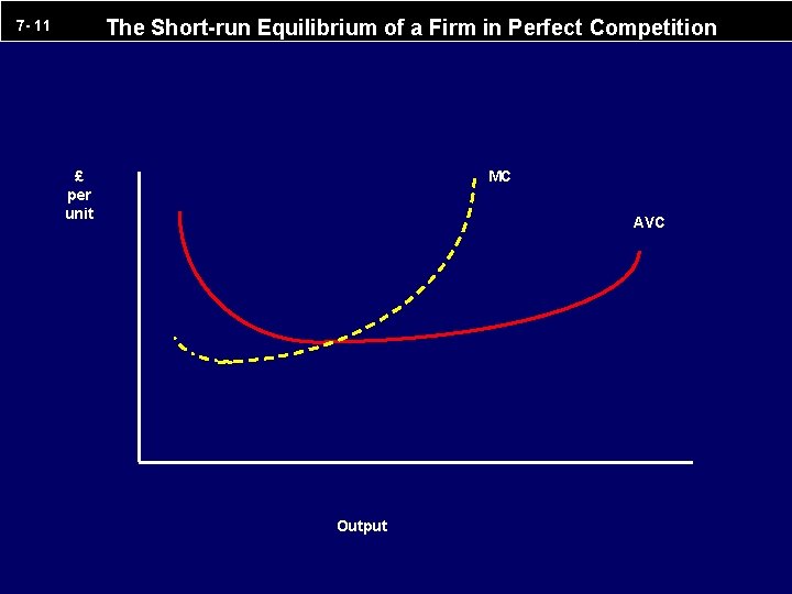
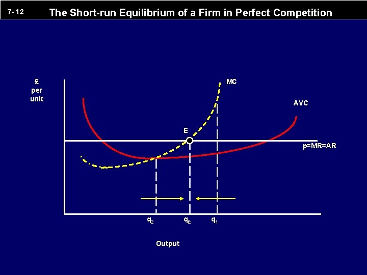
7 - 13 The Short-run Equilibrium of a Firm in Perfect Competition · The firm chooses the output for which p=MC above the level of AVC. · When price equals marginal cost, as at output q. E, the firm loses profits if it either increases or decreases its output. · At any point left of q. E, say q 2, price is greater than the marginal cost, and it pays to increase output (as indicated by the left-hand arrow). · At any point to the right of q. E, say q 1, price is less than the marginal cost, and it pays to reduce output (as indicated by the right-hand arrow).

Total Cost and Revenue Curves 7 - 14 TC £ 0 q. E Output TR

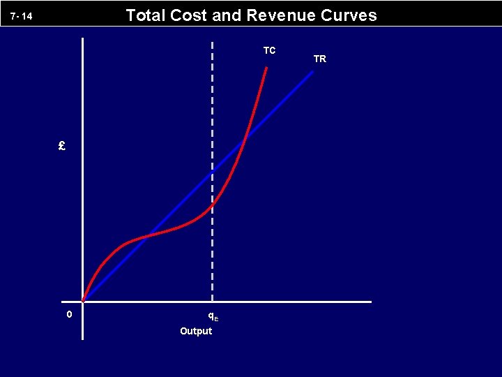
7 - 15 Total Cost and Revenue Curves · At each output the vertical distance between the TR and TC curves shows by how much total revenue exceeds or falls short of total cost. · The gap is largest at output q. E which is the profitmaximizing output.

The Supply Curve for a Price-taking Firm 7 - 16 5 5 4 4 AVC 3 E 0 Price [£] £ per nut MC p 0 2 1 3 2 1 Output [i] Marginal cost and average variable cost curves q 0 Quantity [ii] The supply curve

The Supply Curve for a Price-taking Firm 7 - 17 5 5 4 4 AVC E 1 3 E 0 p 1 Price [£] £ per nut MC p 0 2 1 3 2 1 Output [i] Marginal cost and average variable cost curves q 0 q 1 Quantity [ii] The supply curve

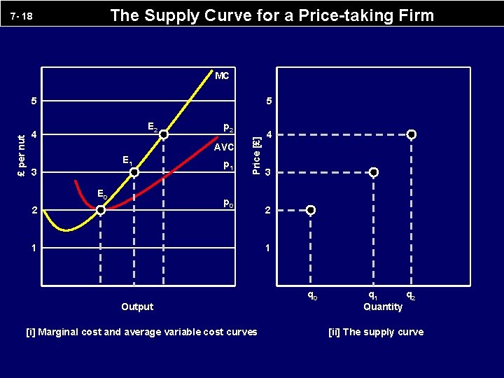
The Supply Curve for a Price-taking Firm 7 - 18 MC 5 E 2 4 p 2 AVC E 1 3 E 0 p 1 Price [£] £ per nut 5 p 0 2 1 4 3 2 1 Output [i] Marginal cost and average variable cost curves q 0 q 1 q 2 Quantity [ii] The supply curve

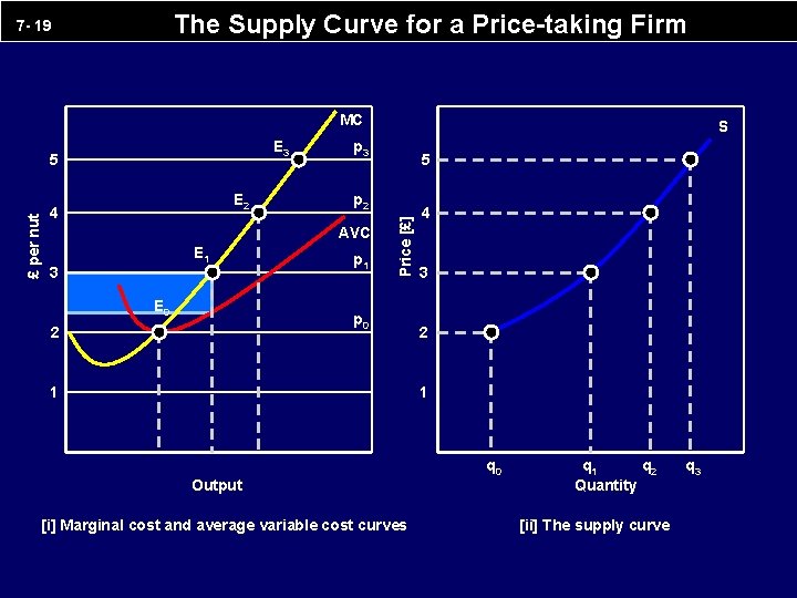
The Supply Curve for a Price-taking Firm 7 - 19 MC £ per nut E 2 4 p 3 p 2 AVC E 1 3 E 0 5 p 1 Price [£] E 3 5 S p 0 2 1 4 3 2 1 Output [i] Marginal cost and average variable cost curves q 0 q 1 q 2 Quantity [ii] The supply curve q 3

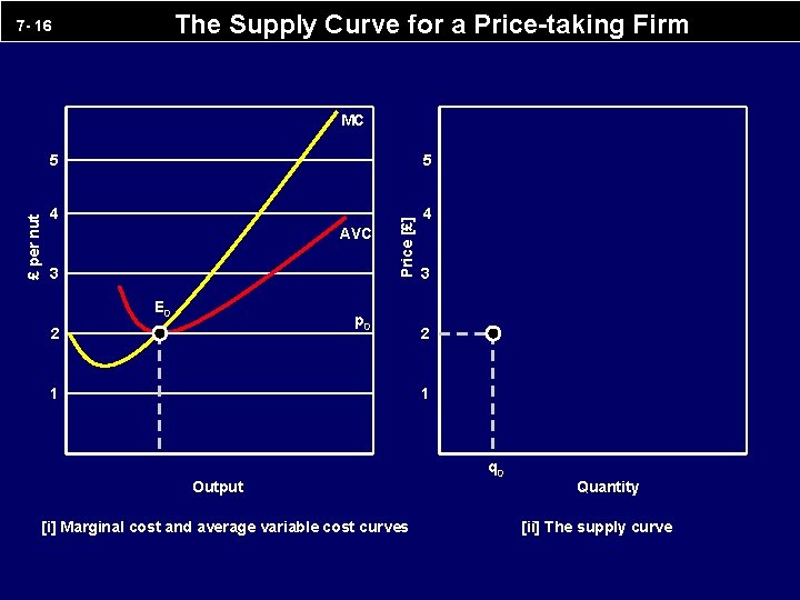
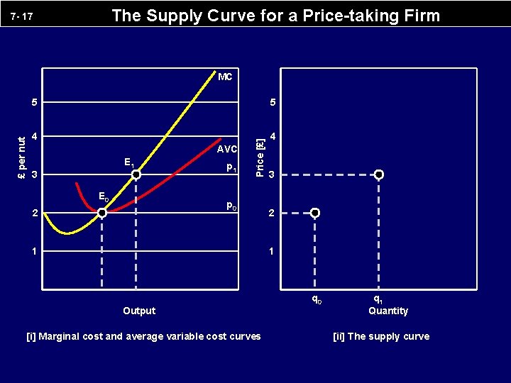
7 - 20 The Supply Curve for a Price-taking Firm · For a price-taking firm the supply curve has the same shape as its MC curve above the level of AVC. · The point E 0, where price, p 0, equals AVC is the shutdown point. · As price rises from £ 2 to £ 3 to £ 4 to £ 5, the firm increases its production from q 0 to q 1 to q 2 to q 3. · For example at a price of £ 3, the firm produces output q 1 and earns the contribution to fixed costs shown by the dark blue shaded rectangle. · The firm’s supply curve is shown in part (ii). · It relates market price to the quantity the firm will produce and offer for sale. · It has the same shape as the firm’s MC curve for all prices above AVC.

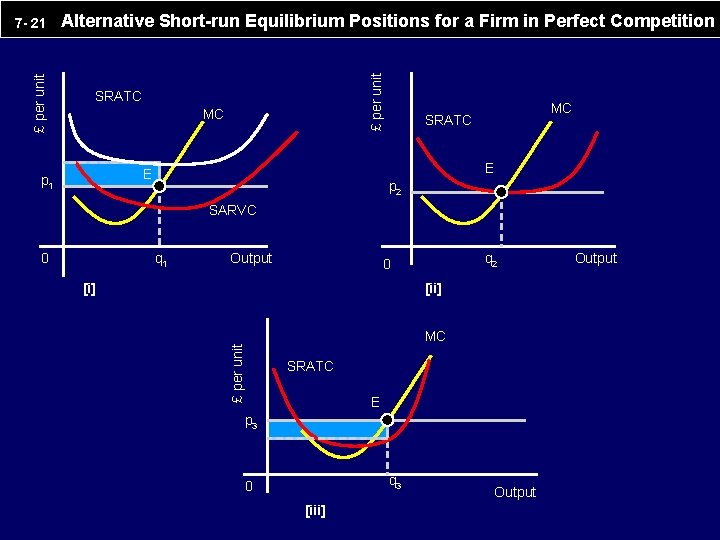
Alternative Short-run Equilibrium Positions for a Firm in Perfect Competition £ per unit 7 - 21 SRATC MC E E p 1 MC SRATC p 2 SARVC 0 q 1 Output q 2 0 [i] [ii] £ per unit MC SRATC E p 3 q 3 0 [iii] Output

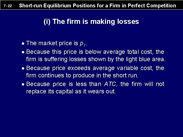
7 - 22 Short-run Equilibrium Positions for a Firm in Perfect Competition (i) The firm is making losses · The market price is p 1. · Because this price is below average total cost, the firm is suffering losses shown by the light blue area. · Because price exceeds average variable cost, the firm continues to produce in the short run. · Because price is less than ATC, the firm will not replace its capital as it wears out.

7 - 23 Short-run Equilibrium Positions for a Firm in Perfect Competition (ii) The firm is just covering all its costs · The market price is p 2. · The firm is just covering its total costs. · It will replace its capital as it wears out since its revenue is covering the full opportunity cost of its capital.

7 - 24 Short-run Equilibrium Positions for a Firm in Perfect Competition (iii) The firm is making pure profits · The market price is p 3. · The firm is earning pure (or economic) profits in excess of all its costs, as shown by the dark blue area. · The firm will replace its capital as it wears out.

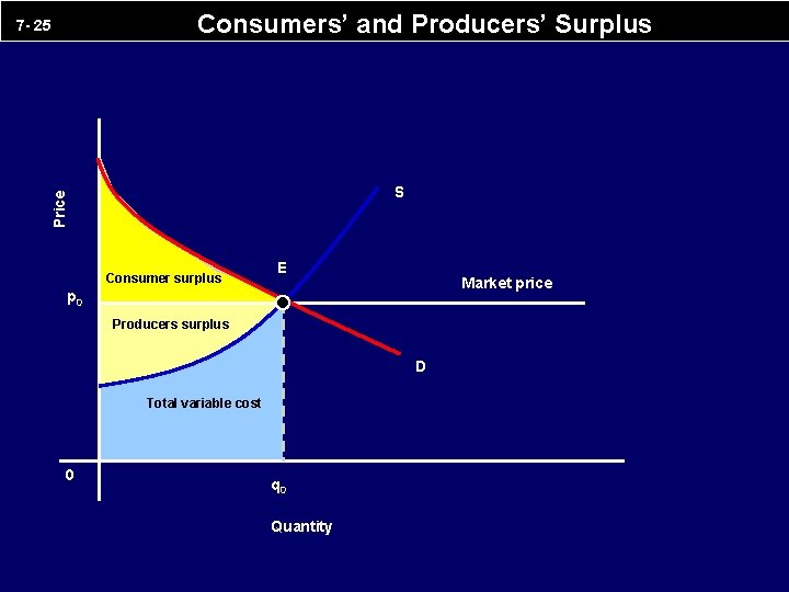
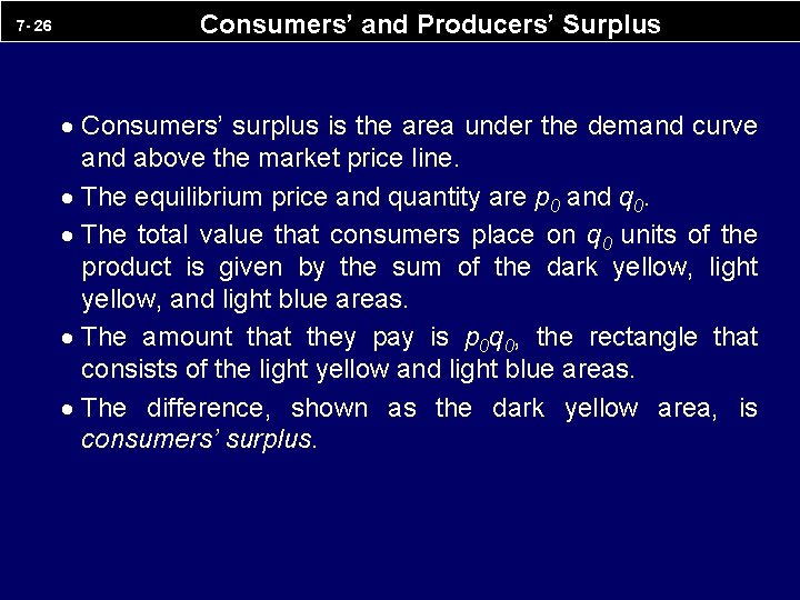
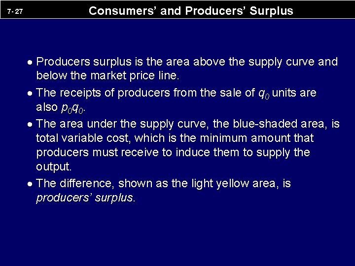
Consumers’ and Producers’ Surplus S Price 7 - 25 Consumer surplus E Market price p 0 Producers surplus D Total variable cost 0 q 0 Quantity

7 - 26 Consumers’ and Producers’ Surplus · Consumers’ surplus is the area under the demand curve and above the market price line. · The equilibrium price and quantity are p 0 and q 0. · The total value that consumers place on q 0 units of the product is given by the sum of the dark yellow, light yellow, and light blue areas. · The amount that they pay is p 0 q 0, the rectangle that consists of the light yellow and light blue areas. · The difference, shown as the dark yellow area, is consumers’ surplus.

7 - 27 Consumers’ and Producers’ Surplus · Producers surplus is the area above the supply curve and below the market price line. · The receipts of producers from the sale of q 0 units are also p 0 q 0. · The area under the supply curve, the blue-shaded area, is total variable cost, which is the minimum amount that producers must receive to induce them to supply the output. · The difference, shown as the light yellow area, is producers’ surplus.

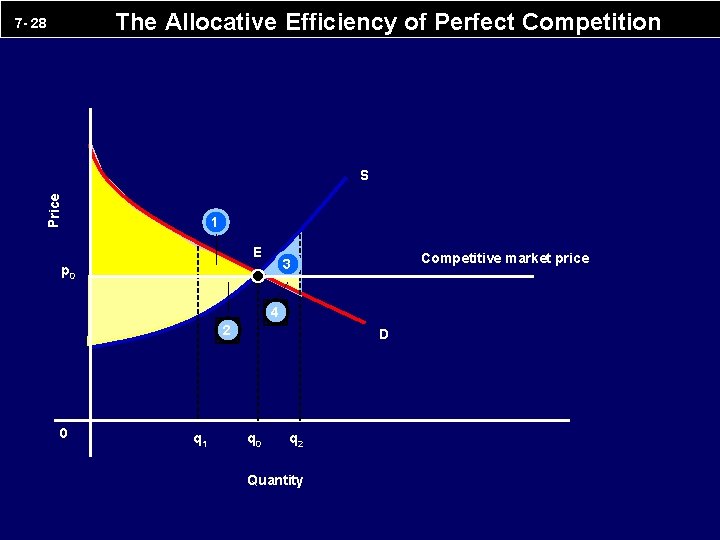
The Allocative Efficiency of Perfect Competition 7 - 28 Price S 1 E Competitive market price 3 p 0 4 2 0 q 1 D q 0 q 2 Quantity

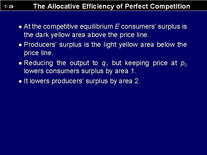
7 - 29 The Allocative Efficiency of Perfect Competition · At the competitive equilibrium E consumers’ surplus is the dark yellow area above the price line. · Producers’ surplus is the light yellow area below the price line. · Reducing the output to q 1 but keeping price at p 0 lowers consumers surplus by area 1. · It lowers producers’ surplus by area 2.

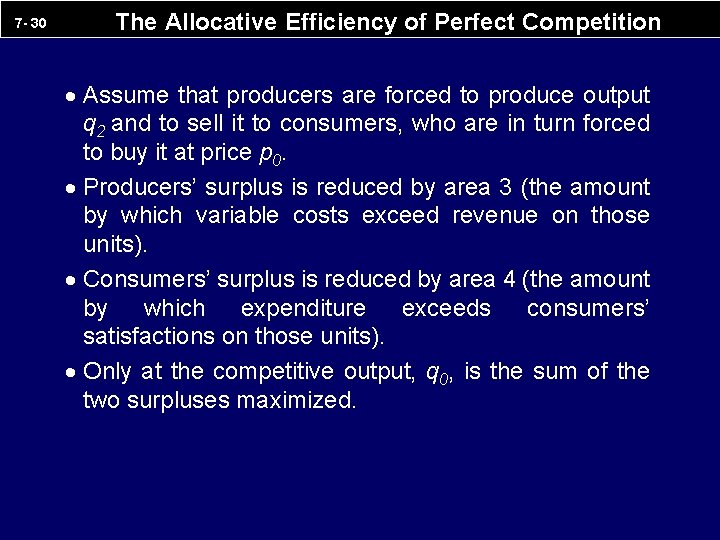
7 - 30 The Allocative Efficiency of Perfect Competition · Assume that producers are forced to produce output q 2 and to sell it to consumers, who are in turn forced to buy it at price p 0. · Producers’ surplus is reduced by area 3 (the amount by which variable costs exceed revenue on those units). · Consumers’ surplus is reduced by area 4 (the amount by which expenditure exceeds consumers’ satisfactions on those units). · Only at the competitive output, q 0, is the sum of the two surpluses maximized.

Short-run and Long-run Equilibrium of a Firm in Perfect Competition 7 - 31 £ per unit SRATC 0 MC 0 p 0 MC* c 0 SRATC* LRAC p* 0 q*

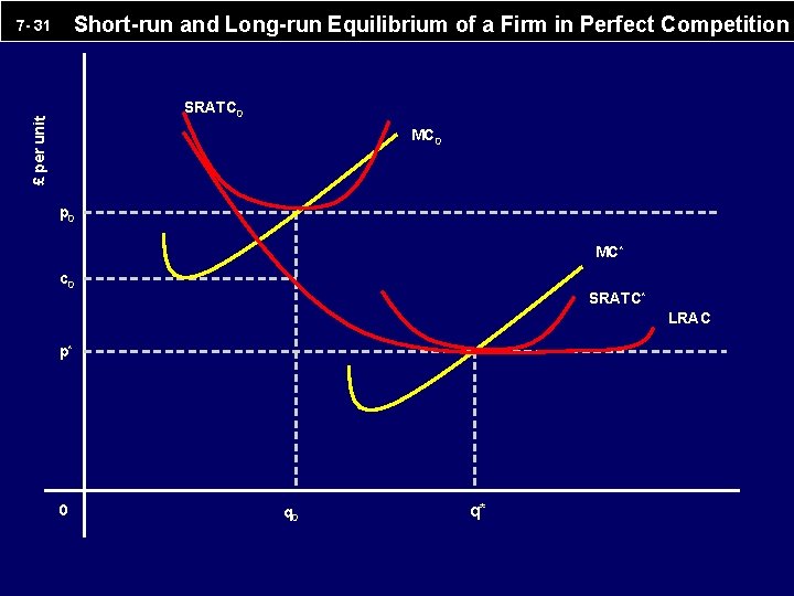
7 - 32 Short-run and Long-run Equilibrium of a Firm in Perfect Competition · The firm’s existing plant has short-run cost curves SRATC 0 and MC 0 while market price is p 0. · The firm produces q 0, where MC 0 equals price and total costs are just being covered. · Although the firm is in short-run equilibrium, it can earn profits by building a larger plant and so moving downwards along its LRAC curve.

7 - 33 Short-run and Long-run Equilibrium of a Firm in Perfect Competition · Thus the firm cannot be in long-run equilibrium at any output below q*, because average total costs can be reduced by building a larger plant. · If all firms do this, industry output will increase and price will fall until long-run equilibrium is reached at price p*. · Each firm is then in short-run equilibrium with a plant whose average cost curve is SRATC* and whose shortrun marginal cost curve, MC*, intersects the price line p at an output of q*. · Because the LRAC curve lies above p* everywhere except at q*, the firm has no incentive to move to another point on its LRAC curve by altering the size of its plant. • Thus a perfectly competitive firm that is not at the minimum point on its LRAC curve cannot be in long-run equilibrium.

Long-run Industry Supply Curves 7 - 34 S 0 Price S 0 Quantity Price D 0 Quantity

Long-run Industry Supply Curves D 0 S 0 E 0 Price p 0 S 0 D 0 q 1 p 0 q 1 Quantity S 0 D 0 Price 7 - 35 p 0 E 0 q 1 Quantity

Long-run Industry Supply Curves D 0 D 1 D 0 E 1 S 0 E 1 p 0 E 0 S 0 Price 7 - 36 q 1 Price D 0 p 0 E 0 q 1 D 1 Quantity p 0 S 0 E 1 E 0 q 1 Quantity

Long-run Industry Supply Curves D 0 D 1 D 0 E 1 S 0 E 2 p 0 E 2 LRS p 0 E 0 p 0 = p 2 E 0 S 0 Price 7 - 37 q 1 D 1 Quantity D 0 Price (i) q 2 p 0 S 0 (ii) Quantity E 1 E 0 E 2 p 0 LRS (iii) q 1 Quantity q 2 LRS

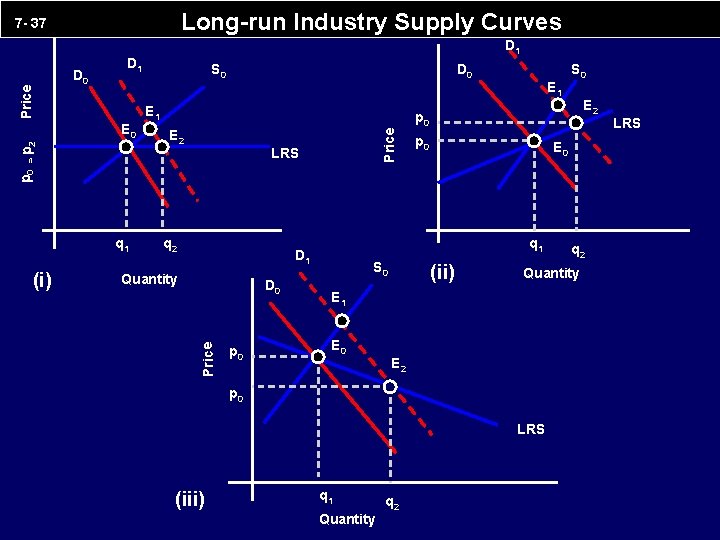
7 - 38 (i) A constant long-run industry supply curve · The initial curves are at D 0 and S 0. · Equilibrium is at E 0 with price p 0 and quantity q 0. · A rise in demand shifts the demand curve to D 1, taking the short-run equilibrium to E 1. · New firms now enter the industry, shifting the short-run supply curve outwards. · Price is pushed down until pure profits are no longer being earned. · At this point the supply curve is S 1. · The new equilibrium is E 2 with price at p 2 and quantity q 2. · The curves shift so that price returns to its original level, making the long-run supply curve horizontal.

7 - 39 (ii) A Rising long-run industry supply curve · The initial curves are at D 0 and S 0. · Equilibrium is at E 0 with price p 0 and quantity q 0. · A rise in demand shifts the demand curve to D 1, taking the short-run equilibrium to E 1. · New firms now enter the industry, shifting the short-run supply curve outwards. · Price is pushed down until pure profits are no longer being earned. · At this point the supply curve is S 1. · The new equilibrium is E 2 with price at p 2 and quantity q 2. · Profits are eliminated and entry ceases before price falls to its original level, giving the LRS curve a positive slope.

7 - 40 (iii) A falling long-run industry supply curve · The initial curves are at D 0 and S 0. · Equilibrium is at E 0 with price p 0 and quantity q 0. · A rise in demand shifts the demand curve to D 1, taking the short-run equilibrium to E 1. · New firms now enter the industry, shifting the short-run supply curve outwards. · Price is pushed down until pure profits are no longer being earned. · At this point the supply curve is S 1. · The new equilibrium is E 2 with price at p 2 and quantity q 2. · The price falls below its original level before profits return to normal, giving the LRS curve a negative slope.

7 - 41 CHAPTER 7: PERFECT COMPETITION Market Structure and Firm Behaviour • Competitive behaviour refers to the extent to which individual firms compete with each other to sell their products. • Competitive market structure refers to the power that individual firms have over the market - perfect competition occurring where firms have no market power and hence no need to react to each other. Perfectly Competitive Markets • The theory of perfect competition is based on the following assumptions: firms sell a homogenous product; customers are well informed; each firm is a price-taker; the industry can support many firms, which are free to enter or leave the industry.

7 - 42 CHAPTER 7: PERFECT COMPETITION Short-run Equilibrium • Any firm maximises profits producing the output where its marginal cost curve intersects the marginal revenue curve from below - or by producing nothing if average cost exceeds price at all outputs. • A perfectly competitive firm is a quantity-adjuster, facing a perfectly elastic demand curve at the given market price and maximising profits by choosing the output that equates its marginal cost to price. • The supply curve of a firm in perfect competition is its marginal cost curve, and the supply curve of a perfectly competitive industry is the sum of the marginal cost curves of all its firms. • The intersection of this curve with the market demand curve for the industry’s product determines market price.

7 - 43 CHAPTER 7: PERFECT COMPETITION Long-run Equilibrium • Long-run industry equilibrium requires that each individual firm be producing at the minimum point of its LRAC curve and be making zero profits. • The long-run industry supply curve for a perfectly competitive industry may be [i] positively sloped, if input prices are driven up by the industry’s expansion, [ii] horizontal, if plants can be replicated and factor prices remain constant, or [iii] negatively sloped, if some other industry that is not perfectly competitive produces an input under conditions of falling long-run costs. The Allocative Efficiency of Perfect Competition • Perfect competition produces an optimal allocation of resources because it maximises the sum of consumers’ and producers’ surplus by producing equilibrium where marginal cost equals price.