1 DistanceVector and PathVector Routing Sections 4 2

1 Distance-Vector and Path-Vector Routing Sections 4. 2. 2. , 4. 3. 2, 4. 3. 3 COS 461: Computer Networks Spring 2011 Mike Freedman http: //www. cs. princeton. edu/courses/archive/spring 11/cos 461/

2 Goals of Today’s Lectures • Distance-vector routing – Pro: Less information than link state – Con: Slower convergence • Path-vector routing – Faster convergence than distance vector – More flexibility in selecting paths • Different goals / metrics if inter- or intra-domain

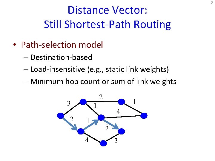
Distance Vector: Still Shortest-Path Routing • Path-selection model – Destination-based – Load-insensitive (e. g. , static link weights) – Minimum hop count or sum of link weights 2 3 2 1 1 1 4 4 5 3 3

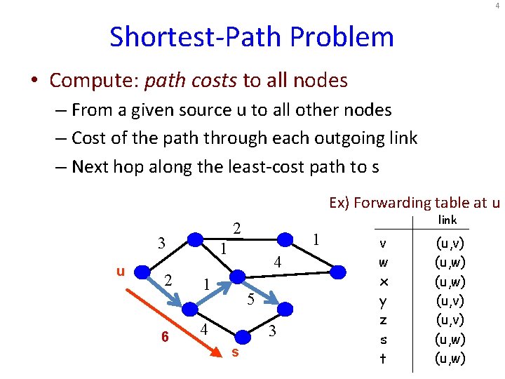
4 Shortest-Path Problem • Compute: path costs to all nodes – From a given source u to all other nodes – Cost of the path through each outgoing link – Next hop along the least-cost path to s Ex) Forwarding table at u 2 3 u 2 6 link 1 1 4 1 5 4 3 s v w x y z s t (u, v) (u, w)

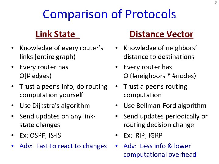
5 Comparison of Protocols Link State • Knowledge of every router’s links (entire graph) • Every router has O(# edges) • Trust a peer’s info, do routing computation yourself • Use Dijkstra’s algorithm • Send updates on any linkstate changes • Ex: OSPF, IS-IS • Adv: Fast to react to changes Distance Vector • Knowledge of neighbors’ distance to destinations • Every router has O (#neighbors * #nodes) • Trust a peer’s routing computation • Use Bellman-Ford algorithm • Send updates periodically or routing decision change • Ex: RIP, IGRP • Adv: Less info & lower computational overhead

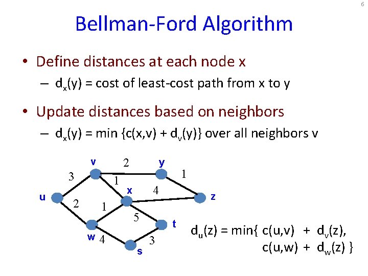
6 Bellman-Ford Algorithm • Define distances at each node x – dx(y) = cost of least-cost path from x to y • Update distances based on neighbors – dx(y) = min {c(x, v) + dv(y)} over all neighbors v 2 v 3 u 1 2 1 w 4 y 1 4 x 5 s z t 3 du(z) = min{ c(u, v) + dv(z), c(u, w) + dw(z) }

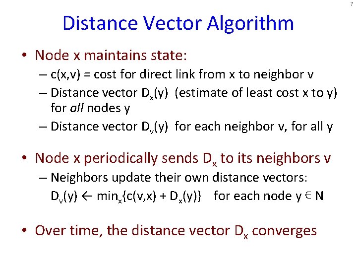
7 Distance Vector Algorithm • Node x maintains state: – c(x, v) = cost for direct link from x to neighbor v – Distance vector Dx(y) (estimate of least cost x to y) for all nodes y – Distance vector Dv(y) for each neighbor v, for all y • Node x periodically sends Dx to its neighbors v – Neighbors update their own distance vectors: Dv(y) ← minx{c(v, x) + Dx(y)} for each node y ∊ N • Over time, the distance vector Dx converges

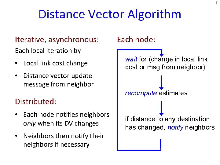
8 Distance Vector Algorithm Iterative, asynchronous: Each node: Each local iteration by • Local link cost change wait for (change in local link cost or msg from neighbor) • Distance vector update message from neighbor Distributed: • Each node notifies neighbors only when its DV changes • Neighbors then notify their neighbors if necessary recompute estimates if distance to any destination has changed, notify neighbors

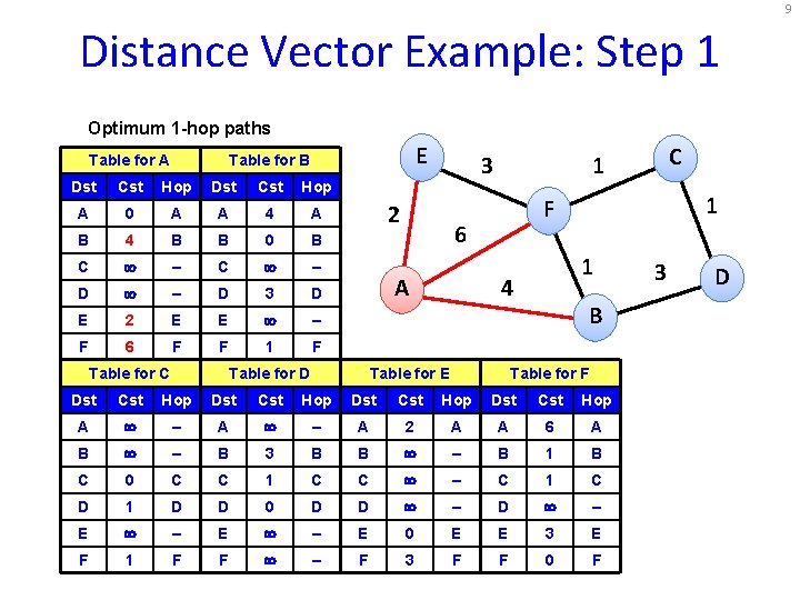
9 Distance Vector Example: Step 1 Optimum 1 -hop paths Table for A E Table for B Dst Cst Hop A 0 A A 4 A B 4 B B 0 B C – D – D 3 D E 2 E E – F 6 F F 1 F Table for C 3 2 Table for D 1 F 6 A C 1 1 4 Table for E B Table for F Dst Cst Hop A – A 2 A A 6 A B – B 3 B B – B 1 B C 0 C C 1 C C – C 1 C D 1 D D 0 D D – E – E 0 E E 3 E F 1 F F – F 3 F F 0 F 3 D

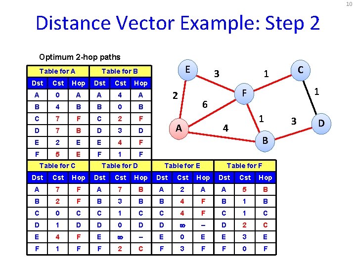
10 Distance Vector Example: Step 2 Optimum 2 -hop paths Table for A E Table for B Dst Cst Hop A 0 A A 4 A B 4 B B 0 B C 7 F C 2 F D 7 B D 3 D E 2 E E 4 F F 5 E F 1 F Table for C 3 2 Table for D 1 F 6 A C 1 1 4 Table for E B Table for F Dst Cst Hop A 7 F A 7 B A 2 A A 5 B B 2 F B 3 B B 4 F B 1 B C 0 C C 1 C C 4 F C 1 C D 1 D D 0 D D – D 2 C E 4 F E – E 0 E E 3 E F 1 F F 2 C F 3 F F 0 F 3 D

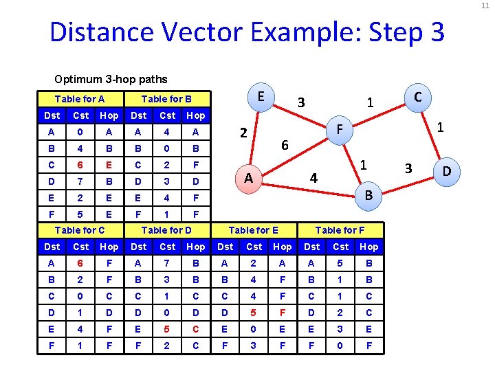
11 Distance Vector Example: Step 3 Optimum 3 -hop paths Table for A E Table for B Dst Cst Hop A 0 A A 4 A B 4 B B 0 B C 6 E C 2 F D 7 B D 3 D E 2 E E 4 F F 5 E F 1 F Table for C 3 2 Table for D 1 F 6 A C 1 1 4 Table for E B Table for F Dst Cst Hop A 6 F A 7 B A 2 A A 5 B B 2 F B 3 B B 4 F B 1 B C 0 C C 1 C C 4 F C 1 C D 1 D D 0 D D 5 F D 2 C E 4 F E 5 C E 0 E E 3 E F 1 F F 2 C F 3 F F 0 F 3 D

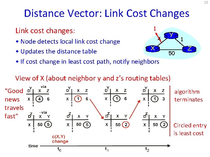
12 Distance Vector: Link Cost Changes Link cost changes: 1 4 • Node detects local link cost change X • Updates the distance table • If cost change in least cost path, notify neighbors Y 1 50 Z View of X (about neighbor y and z’s routing tables) “Good news travels fast” algorithm terminates Circled entry is least cost

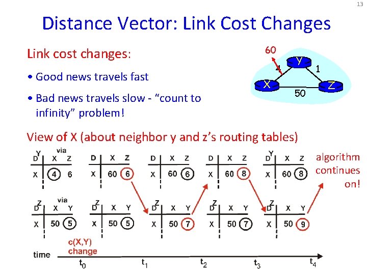
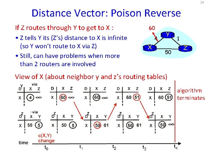
13 Distance Vector: Link Cost Changes Link cost changes: • Good news travels fast • Bad news travels slow - “count to infinity” problem! 60 4 X Y 50 1 Z View of X (about neighbor y and z’s routing tables) algorithm continues on!

14 Distance Vector: Poison Reverse If Z routes through Y to get to X : • Z tells Y its (Z’s) distance to X is infinite (so Y won’t route to X via Z) • Still, can have problems when more than 2 routers are involved 60 4 X Y 50 1 Z View of X (about neighbor y and z’s routing tables) algorithm terminates

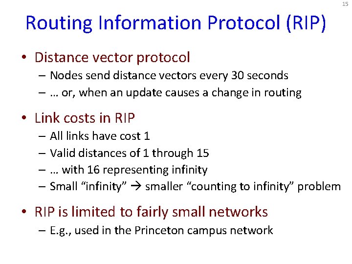
15 Routing Information Protocol (RIP) • Distance vector protocol – Nodes send distance vectors every 30 seconds – … or, when an update causes a change in routing • Link costs in RIP – All links have cost 1 – Valid distances of 1 through 15 – … with 16 representing infinity – Small “infinity” smaller “counting to infinity” problem • RIP is limited to fairly small networks – E. g. , used in the Princeton campus network

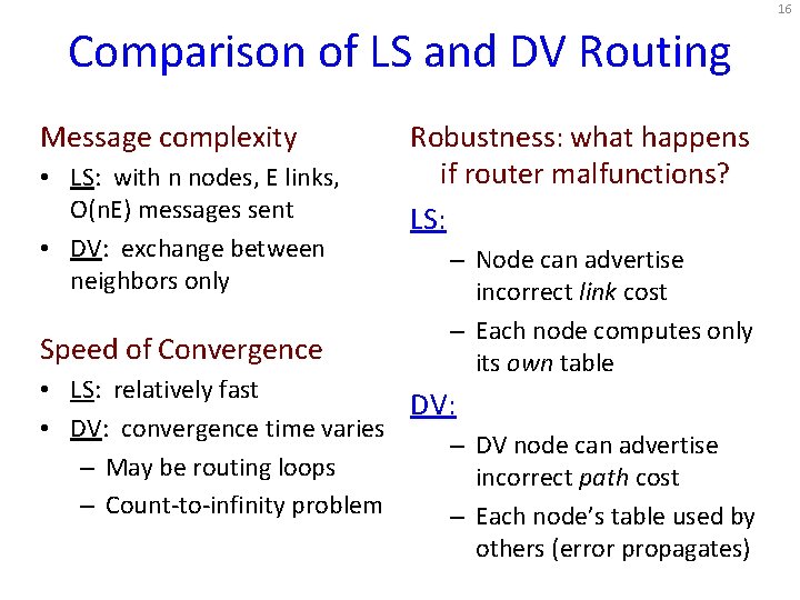
16 Comparison of LS and DV Routing Message complexity • LS: with n nodes, E links, O(n. E) messages sent • DV: exchange between neighbors only Speed of Convergence Robustness: what happens if router malfunctions? LS: – Node can advertise incorrect link cost – Each node computes only its own table • LS: relatively fast DV: • DV: convergence time varies – DV node can advertise – May be routing loops incorrect path cost – Count-to-infinity problem – Each node’s table used by others (error propagates)

17 Similarities of LS and DV Routing • Shortest-path routing – Metric-based, using link weights – Routers share a common view of how good a path is • As such, commonly used inside an organization – RIP and OSPF are mostly used as intra-domain protocols – E. g. , Princeton uses RIP, and AT&T uses OSPF • But the Internet is a “network of networks” – How to stitch the many networks together? – When networks may not have common goals – … and may not want to share information

18 Path-Vector Routing

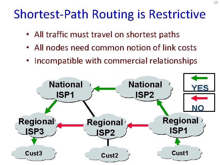
19 Shortest-Path Routing is Restrictive • All traffic must travel on shortest paths • All nodes need common notion of link costs • Incompatible with commercial relationships National ISP 1 Regional ISP 3 Cust 3 National ISP 2 Regional ISP 2 Cust 2 YES NO Regional ISP 1 Cust 1

20 Link-State Routing is Problematic • Topology information is flooded – High bandwidth and storage overhead – Forces nodes to divulge sensitive information • Entire path computed locally per node – High processing overhead in a large network • Minimizes some notion of total distance – Works only if policy is shared and uniform • Typically used only inside an AS – E. g. , OSPF and IS-IS

21 Distance Vector is on the Right Track • Advantages – Hides details of the network topology – Nodes determine only “next hop” toward the dest • Disadvantages – Minimizes some notion of total distance, which is difficult in an interdomain setting – Slow convergence due to the counting-to-infinity problem (“bad news travels slowly”) • Idea: extend the notion of a distance vector – To make it easier to detect loops

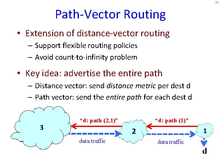
22 Path-Vector Routing • Extension of distance-vector routing – Support flexible routing policies – Avoid count-to-infinity problem • Key idea: advertise the entire path – Distance vector: send distance metric per dest d – Path vector: send the entire path for each dest d 3 “d: path (2, 1)” “d: path (1)” 1 2 data traffic d

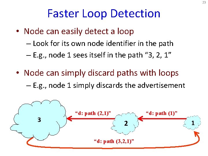
23 Faster Loop Detection • Node can easily detect a loop – Look for its own node identifier in the path – E. g. , node 1 sees itself in the path “ 3, 2, 1” • Node can simply discard paths with loops – E. g. , node 1 simply discards the advertisement 3 “d: path (2, 1)” “d: path (1)” 2 “d: path (3, 2, 1)” 1

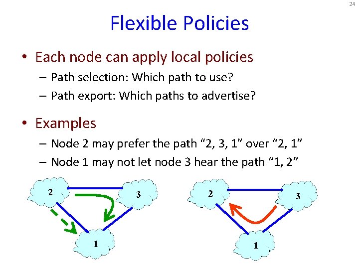
24 Flexible Policies • Each node can apply local policies – Path selection: Which path to use? – Path export: Which paths to advertise? • Examples – Node 2 may prefer the path “ 2, 3, 1” over “ 2, 1” – Node 1 may not let node 3 hear the path “ 1, 2” 2 3 1

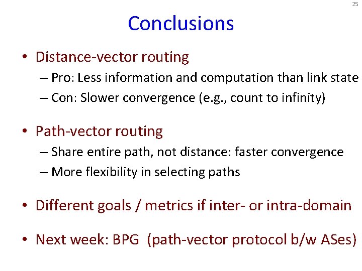
25 Conclusions • Distance-vector routing – Pro: Less information and computation than link state – Con: Slower convergence (e. g. , count to infinity) • Path-vector routing – Share entire path, not distance: faster convergence – More flexibility in selecting paths • Different goals / metrics if inter- or intra-domain • Next week: BPG (path-vector protocol b/w ASes)