030612 Structure from Motion Computer Vision CS 543

03/06/12 Structure from Motion Computer Vision CS 543 / ECE 549 University of Illinois Derek Hoiem Many slides adapted from Lana Lazebnik, Silvio Saverese, Steve Seitz, Martial Hebert

This class: structure from motion • Recap of epipolar geometry – Depth from two views • Projective structure from motion • Affine structure from motion

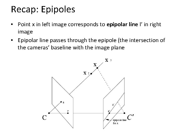
Recap: Epipoles • Point x in left image corresponds to epipolar line l’ in right image • Epipolar line passes through the epipole (the intersection of the cameras’ baseline with the image plane

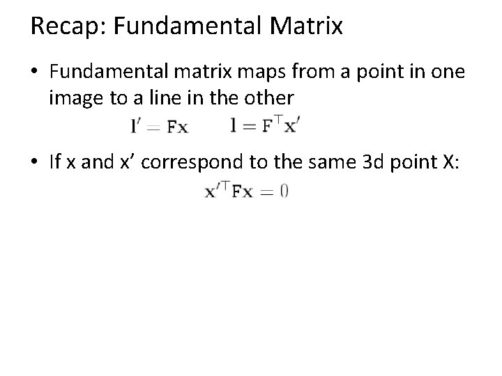
Recap: Fundamental Matrix • Fundamental matrix maps from a point in one image to a line in the other • If x and x’ correspond to the same 3 d point X:

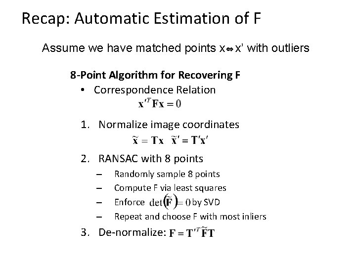
Recap: Automatic Estimation of F Assume we have matched points x x’ with outliers 8 -Point Algorithm for Recovering F • Correspondence Relation 1. Normalize image coordinates 2. RANSAC with 8 points – – Randomly sample 8 points Compute F via least squares Enforce by SVD Repeat and choose F with most inliers 3. De-normalize:

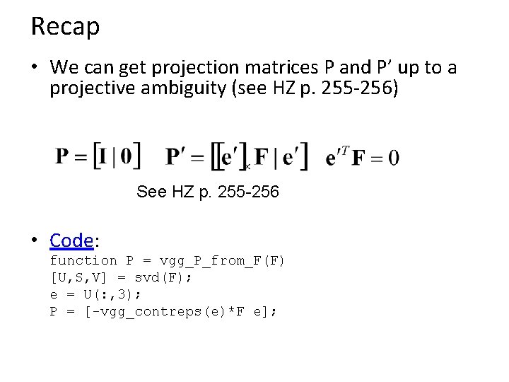
Recap • We can get projection matrices P and P’ up to a projective ambiguity (see HZ p. 255 -256) See HZ p. 255 -256 • Code: function P = vgg_P_from_F(F) [U, S, V] = svd(F); e = U(: , 3); P = [-vgg_contreps(e)*F e];

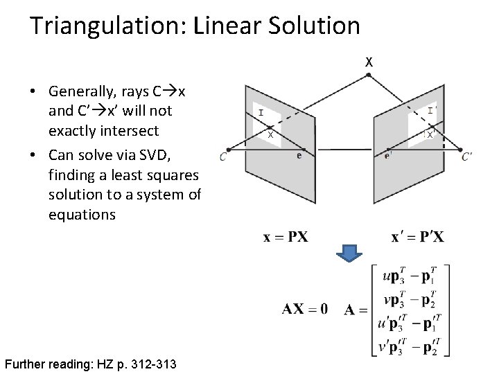
Triangulation: Linear Solution X • Generally, rays C x and C’ x’ will not exactly intersect • Can solve via SVD, finding a least squares solution to a system of equations Further reading: HZ p. 312 -313 x x'

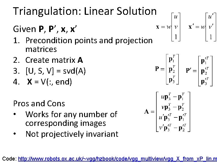
Triangulation: Linear Solution Given P, P’, x, x’ 1. Precondition points and projection matrices 2. Create matrix A 3. [U, S, V] = svd(A) 4. X = V(: , end) Pros and Cons • Works for any number of corresponding images • Not projectively invariant Code: http: //www. robots. ox. ac. uk/~vgg/hzbook/code/vgg_multiview/vgg_X_from_x. P_lin. m

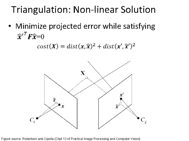
Triangulation: Non-linear Solution • Minimize projected error while satisfying Figure source: Robertson and Cipolla (Chpt 13 of Practical Image Processing and Computer Vision)

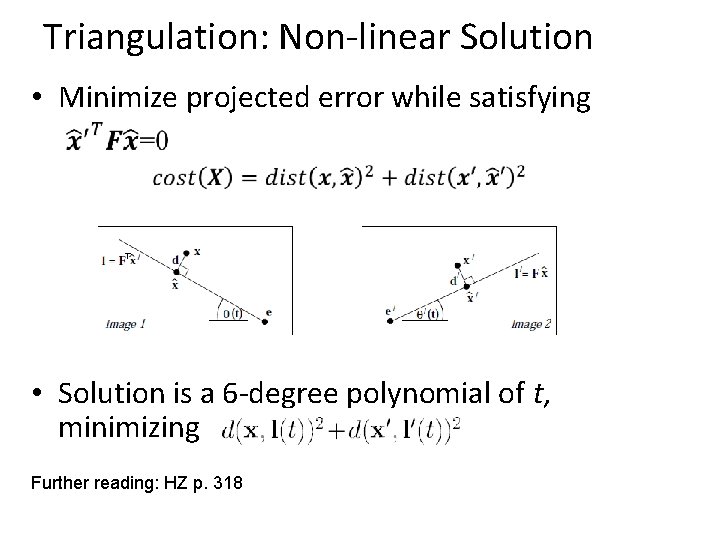
Triangulation: Non-linear Solution • Minimize projected error while satisfying • Solution is a 6 -degree polynomial of t, minimizing Further reading: HZ p. 318

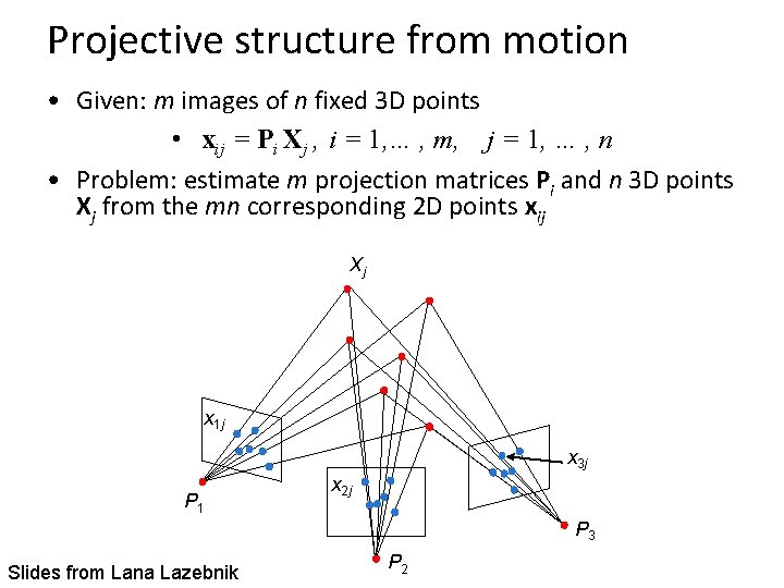
Projective structure from motion • Given: m images of n fixed 3 D points • xij = Pi Xj , i = 1, … , m, j = 1, … , n • Problem: estimate m projection matrices Pi and n 3 D points Xj from the mn corresponding 2 D points xij Xj x 1 j x 3 j P 1 x 2 j P 3 Slides from Lana Lazebnik P 2

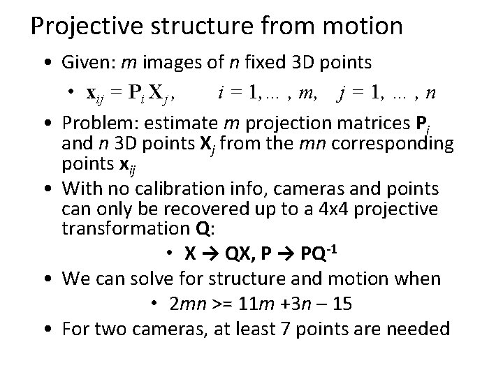
Projective structure from motion • Given: m images of n fixed 3 D points • xij = Pi Xj , i = 1, … , m, j = 1, … , n • Problem: estimate m projection matrices Pi and n 3 D points Xj from the mn corresponding points xij • With no calibration info, cameras and points can only be recovered up to a 4 x 4 projective transformation Q: • X → QX, P → PQ-1 • We can solve for structure and motion when • 2 mn >= 11 m +3 n – 15 • For two cameras, at least 7 points are needed

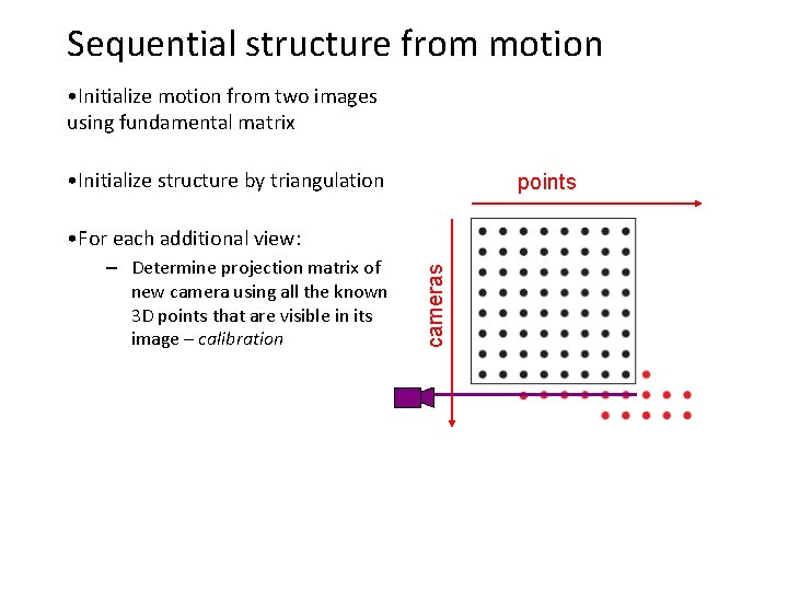
Sequential structure from motion • Initialize motion from two images using fundamental matrix • Initialize structure by triangulation points – Determine projection matrix of new camera using all the known 3 D points that are visible in its image – calibration cameras • For each additional view:

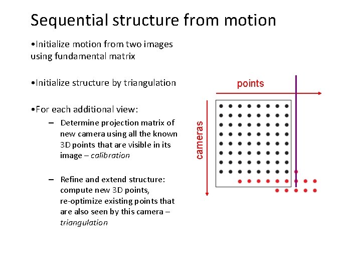
Sequential structure from motion • Initialize motion from two images using fundamental matrix • Initialize structure by triangulation points – Determine projection matrix of new camera using all the known 3 D points that are visible in its image – calibration – Refine and extend structure: compute new 3 D points, re-optimize existing points that are also seen by this camera – triangulation cameras • For each additional view:

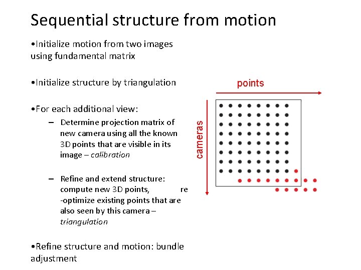
Sequential structure from motion • Initialize motion from two images using fundamental matrix • Initialize structure by triangulation points – Determine projection matrix of new camera using all the known 3 D points that are visible in its image – calibration – Refine and extend structure: compute new 3 D points, re -optimize existing points that are also seen by this camera – triangulation • Refine structure and motion: bundle adjustment cameras • For each additional view:

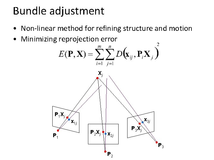
Bundle adjustment • Non-linear method for refining structure and motion • Minimizing reprojection error Xj P 1 x 3 j x 1 j P 2 Xj x 2 j P 3 Xj P 3 P 2

Auto-calibration • Auto-calibration: determining intrinsic camera parameters directly from uncalibrated images • For example, we can use the constraint that a moving camera has a fixed intrinsic matrix – Compute initial projective reconstruction and find 3 D projective transformation matrix Q such that all camera matrices are in the form Pi = K [Ri | ti] • Can use constraints on the form of the calibration matrix, such as zero skew

Summary so far • From two images, we can: – Recover fundamental matrix F – Recover canonical cameras P and P’ from F – Estimate 3 D positions (if K is known) that correspond to each pixel • For a moving camera, we can: – Initialize by computing F, P, X for two images – Sequentially add new images, computing new P, refining X, and adding points – Auto-calibrate assuming fixed calibration matrix to upgrade to similarity transform

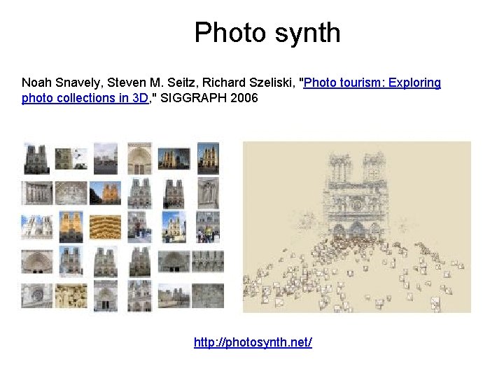
Photo synth Noah Snavely, Steven M. Seitz, Richard Szeliski, "Photo tourism: Exploring photo collections in 3 D, " SIGGRAPH 2006 http: //photosynth. net/

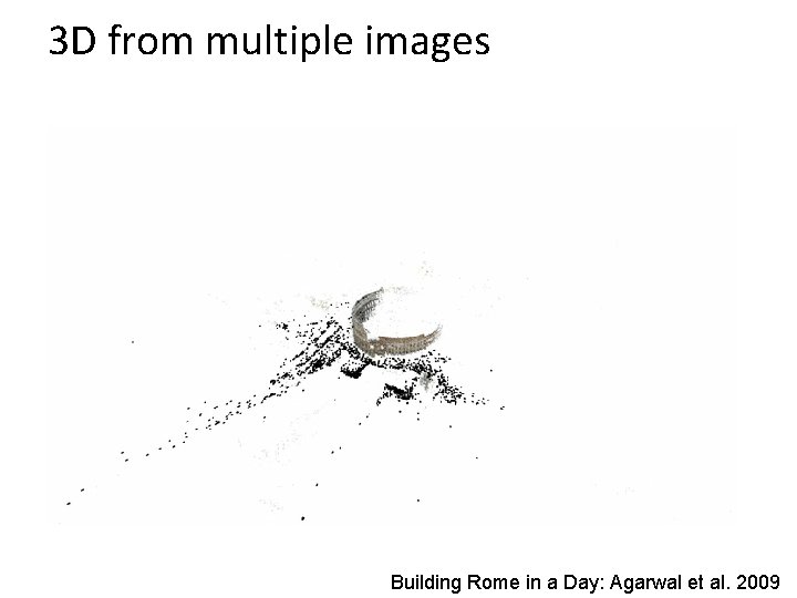
3 D from multiple images Building Rome in a Day: Agarwal et al. 2009

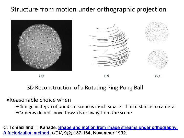
Structure from motion under orthographic projection 3 D Reconstruction of a Rotating Ping-Pong Ball • Reasonable choice when • Change in depth of points in scene is much smaller than distance to camera • Cameras do not move towards or away from the scene C. Tomasi and T. Kanade. Shape and motion from image streams under orthography: A factorization method. IJCV, 9(2): 137 -154, November 1992.

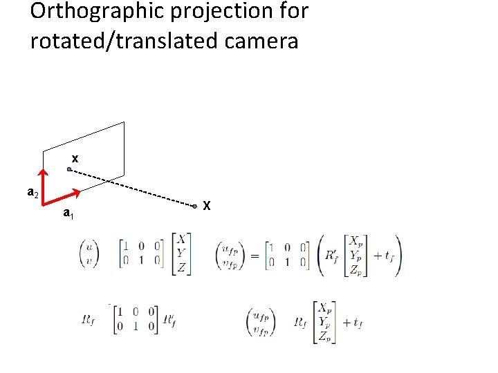
Orthographic projection for rotated/translated camera x a 2 a 1 X

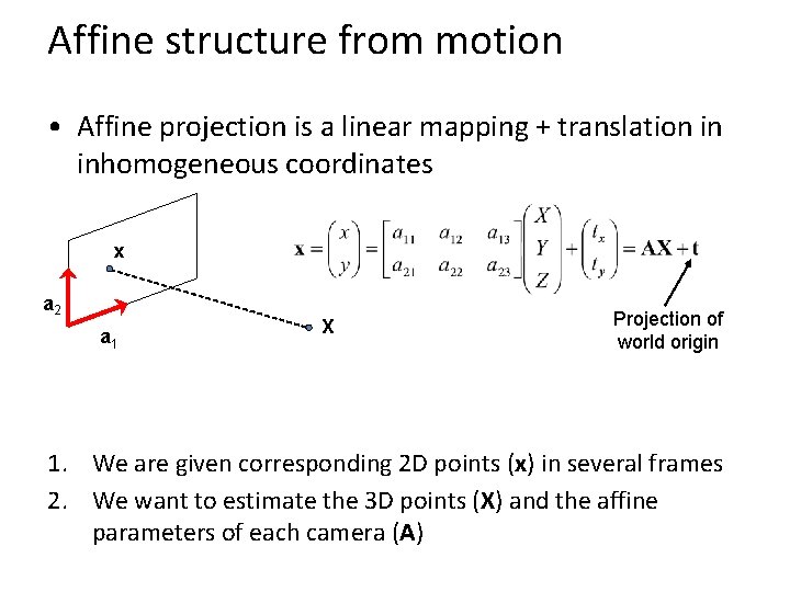
Affine structure from motion • Affine projection is a linear mapping + translation in inhomogeneous coordinates x a 2 a 1 X Projection of world origin 1. We are given corresponding 2 D points (x) in several frames 2. We want to estimate the 3 D points (X) and the affine parameters of each camera (A)

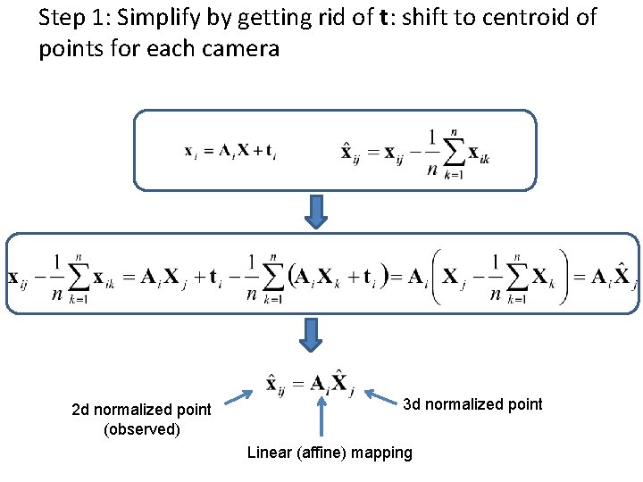
Step 1: Simplify by getting rid of t: shift to centroid of points for each camera 2 d normalized point (observed) 3 d normalized point Linear (affine) mapping

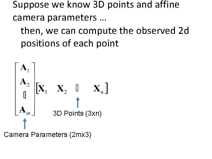
Suppose we know 3 D points and affine camera parameters … then, we can compute the observed 2 d positions of each point 3 D Points (3 xn) Camera Parameters (2 mx 3) 2 D Image Points (2 mxn)

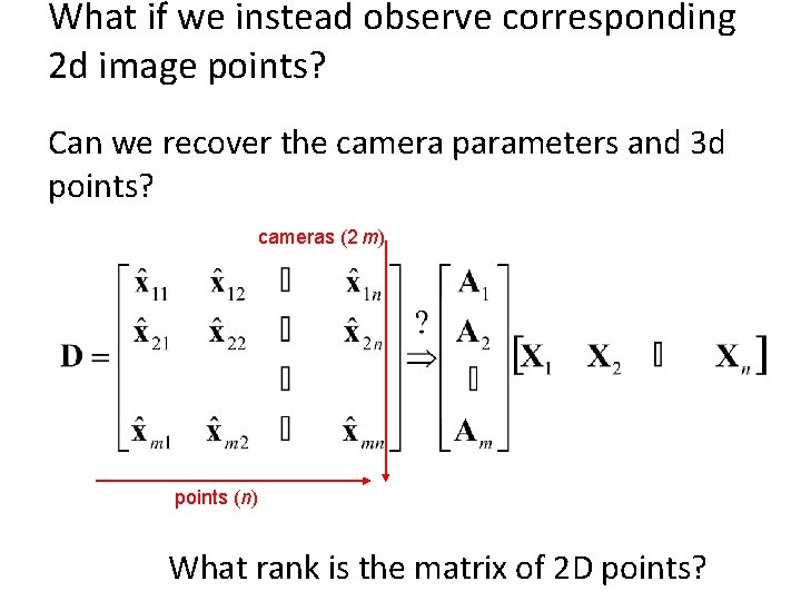
What if we instead observe corresponding 2 d image points? Can we recover the camera parameters and 3 d points? cameras (2 m) points (n) What rank is the matrix of 2 D points?

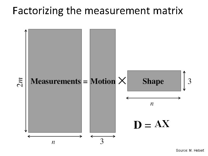
Factorizing the measurement matrix AX Source: M. Hebert

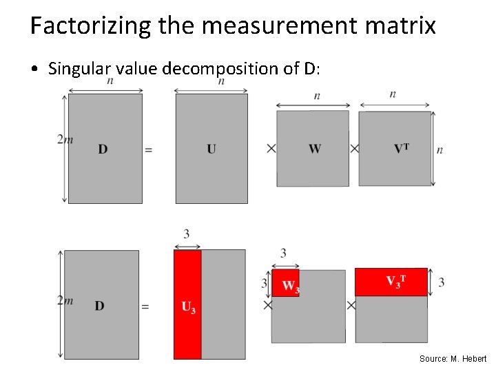
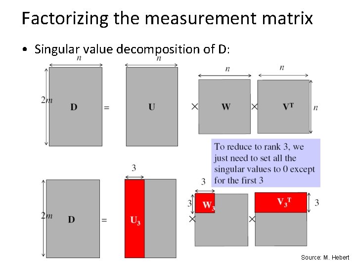
Factorizing the measurement matrix • Singular value decomposition of D: Source: M. Hebert

Factorizing the measurement matrix • Singular value decomposition of D: Source: M. Hebert

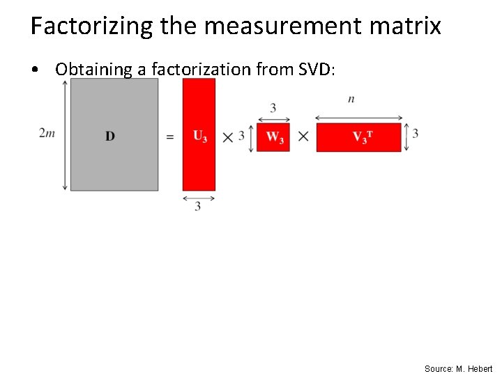
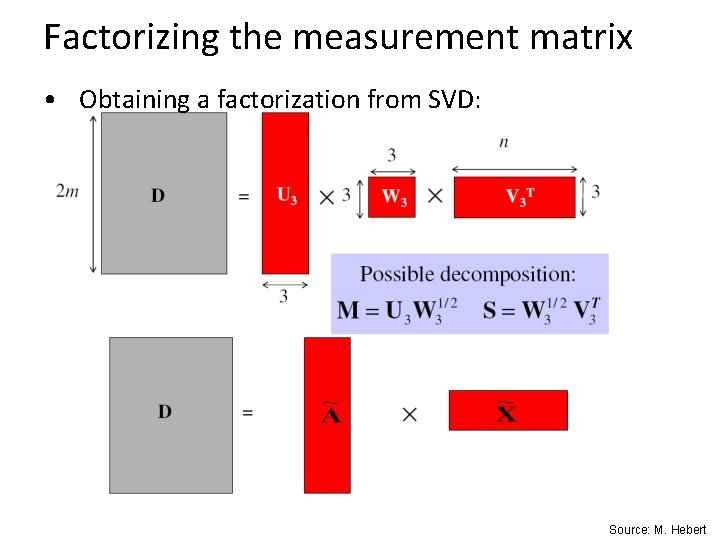
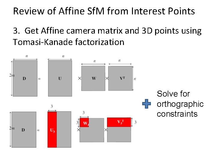
Factorizing the measurement matrix • Obtaining a factorization from SVD: Source: M. Hebert

Factorizing the measurement matrix • Obtaining a factorization from SVD: Source: M. Hebert

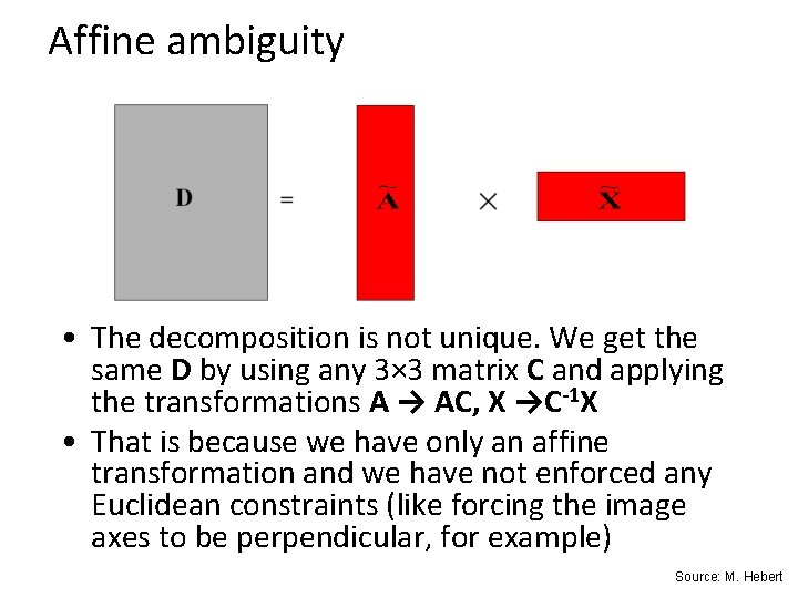
Affine ambiguity • The decomposition is not unique. We get the same D by using any 3× 3 matrix C and applying the transformations A → AC, X →C-1 X • That is because we have only an affine transformation and we have not enforced any Euclidean constraints (like forcing the image axes to be perpendicular, for example) Source: M. Hebert

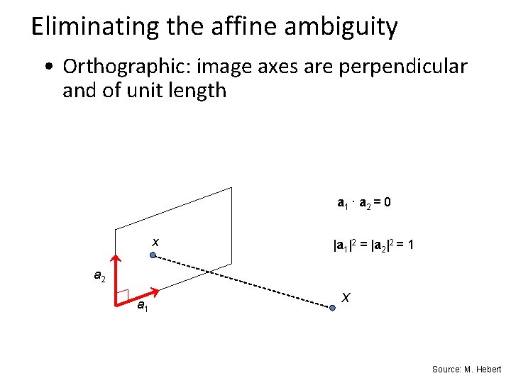
Eliminating the affine ambiguity • Orthographic: image axes are perpendicular and of unit length a 1 · a 2 = 0 x |a 1|2 = |a 2|2 = 1 a 2 a 1 X Source: M. Hebert

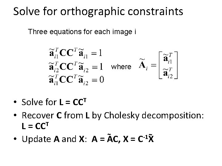
Solve for orthographic constraints Three equations for each image i where • Solve for L = CCT • Recover C from L by Cholesky decomposition: L = CCT ~ ~ -1 • Update A and X: A = AC, X = C X

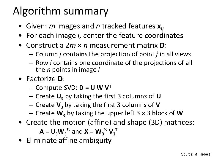
Algorithm summary • Given: m images and n tracked features xij • For each image i, center the feature coordinates • Construct a 2 m × n measurement matrix D: – Column j contains the projection of point j in all views – Row i contains one coordinate of the projections of all the n points in image i • Factorize D: – – Compute SVD: D = U W VT Create U 3 by taking the first 3 columns of U Create V 3 by taking the first 3 columns of V Create W 3 by taking the upper left 3 × 3 block of W • Create the motion (affine) and shape (3 D) matrices: A = U 3 W 3½ and X = W 3½ V 3 T • Eliminate affine ambiguity Source: M. Hebert

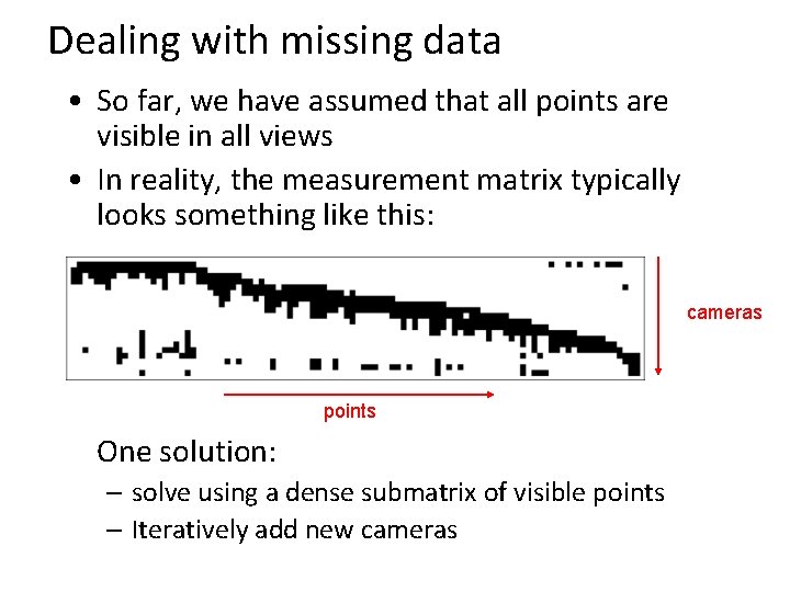
Dealing with missing data • So far, we have assumed that all points are visible in all views • In reality, the measurement matrix typically looks something like this: cameras points One solution: – solve using a dense submatrix of visible points – Iteratively add new cameras

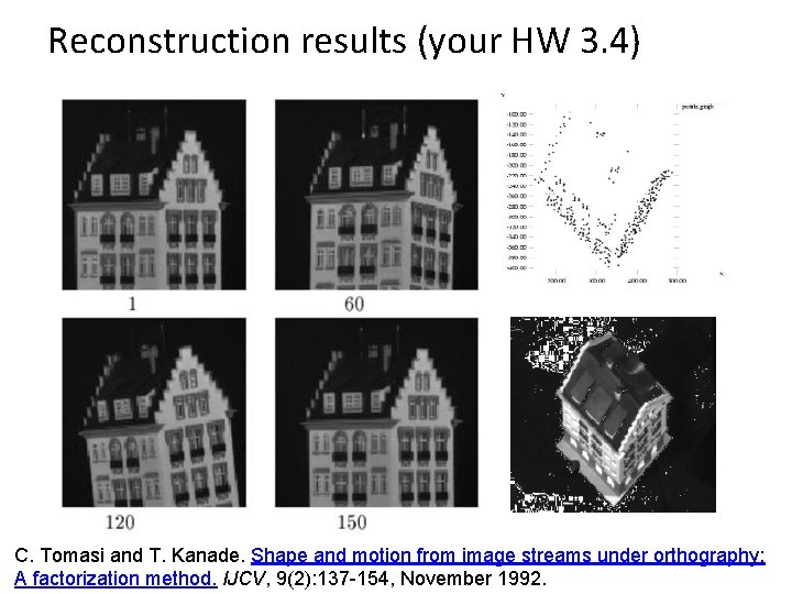
Reconstruction results (your HW 3. 4) C. Tomasi and T. Kanade. Shape and motion from image streams under orthography: A factorization method. IJCV, 9(2): 137 -154, November 1992.

Further reading • Short explanation of Affine Sf. M: class notes from Lischinksi and Gruber http: //www. cs. huji. ac. il/~csip/sfm. pdf • Clear explanation of epipolar geometry and projective Sf. M – http: //mi. eng. cam. ac. uk/~cipolla/publications/contribution. To. Edited. B ook/2008 -SFM-chapters. pdf

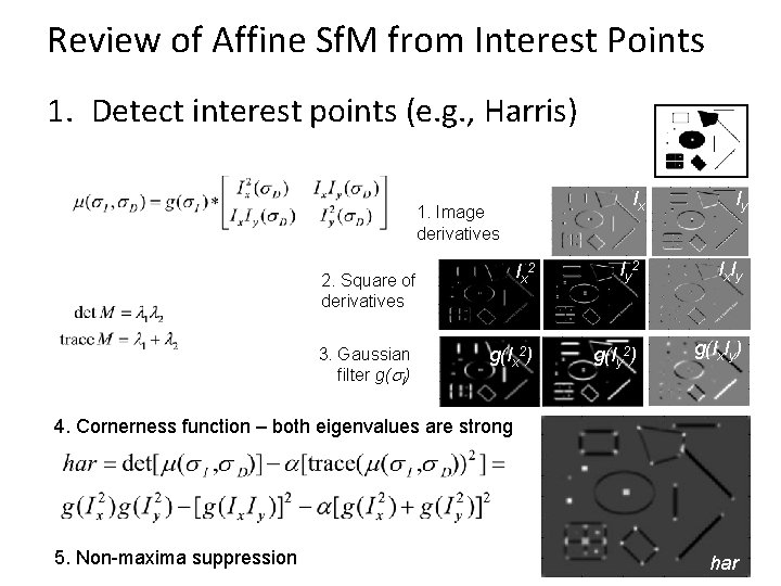
Review of Affine Sf. M from Interest Points 1. Detect interest points (e. g. , Harris) Ix Iy Ix 2 Iy 2 Ix Iy g(Ix 2) g(Iy 2) g(Ix. Iy) 1. Image derivatives 2. Square of derivatives 3. Gaussian filter g(s. I) 4. Cornerness function – both eigenvalues are strong 5. Non-maxima suppression 43 har

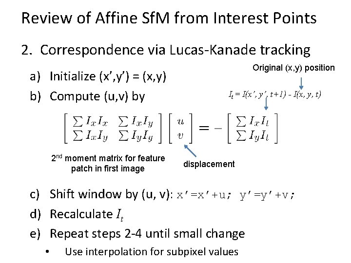
Review of Affine Sf. M from Interest Points 2. Correspondence via Lucas-Kanade tracking a) Initialize (x’, y’) = (x, y) b) Compute (u, v) by 2 nd moment matrix for feature patch in first image Original (x, y) position It = I(x’, y’, t+1) - I(x, y, t) displacement c) Shift window by (u, v): x’=x’+u; y’=y’+v; d) Recalculate It e) Repeat steps 2 -4 until small change • Use interpolation for subpixel values

Review of Affine Sf. M from Interest Points 3. Get Affine camera matrix and 3 D points using Tomasi-Kanade factorization Solve for orthographic constraints

Tips for HW 3 • Problem 1: vanishing points – Use lots of lines to estimate vanishing points – For estimation of VP from lots of lines, see single-view geometry chapter, or use robust estimator of a central intersection point – For obtaining intrinsic camera matrix, numerical solver (e. g. , fsolve in matlab) may be helpful • Problem 3: epipolar geometry – Use reprojection distance for inlier check (make sure to compute line to point distance correctly) • Problem 4: structure from motion – Use Matlab’s chol and svd – If you weren’t able to get tracking to work from HW 2 can use provided points

Distance of point to epipolar line l=Fx=[a b c] . x‘=[u v 1]

Next class • Clustering and using clustered interest points for matching images in a large database