Waiting Line and Queuing Theory Kusdhianto Setiawan Gadjah

Waiting Line and Queuing Theory Kusdhianto Setiawan Gadjah Mada University

Waiting Line Costs • All costs associated with and consequences that come from idleness or the unwillingness to wait from customer can be categorized as waiting cost, inlcuding customer dissatisfaction and lost goodwill

Objectives • Finding the best level of service for an organization that minimizes total expected cost • Total expected cost: the sum of service plus waiting time • Trade-off: the cost of providing good service and the cost of customer waiting time (more difficult to predict)

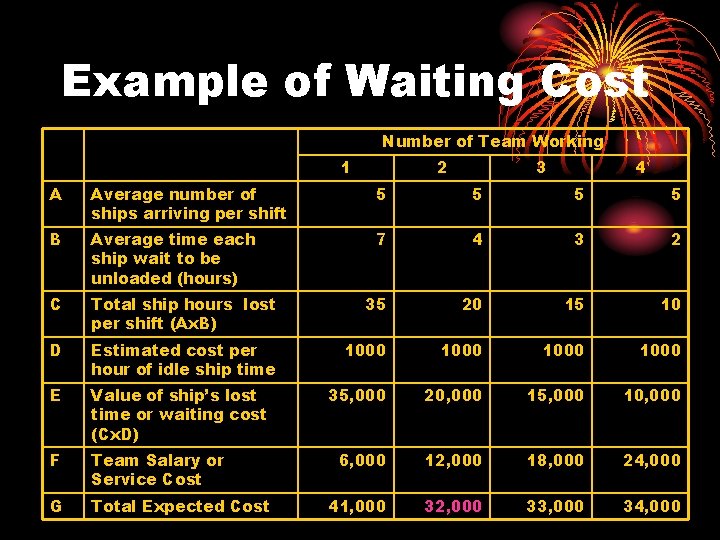
Example of Waiting Cost Number of Team Working 1 2 3 4 A Average number of ships arriving per shift 5 5 B Average time each ship wait to be unloaded (hours) 7 4 3 2 C Total ship hours lost per shift (Ax. B) 35 20 15 10 D Estimated cost per hour of idle ship time 1000 E Value of ship’s lost time or waiting cost (Cx. D) 35, 000 20, 000 15, 000 10, 000 F Team Salary or Service Cost 6, 000 12, 000 18, 000 24, 000 G Total Expected Cost 41, 000 32, 000 33, 000 34, 000

Characteristic of A Queuing System • Arrival Characteristics (calling population) • The Queue or waiting line • The Service Facility All of those must be determined before we develop a model

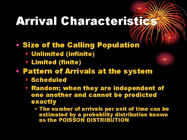
Arrival Characteristics • Size of the Calling Population • Unlimited (infinite) • Limited (finite) • Pattern of Arrivals at the system • Scheduled • Random; when they are independent of one another and cannot be predicted exactly • The number of arrivals per unit of time can be estimated by a probability distribution known as the POISSON DISTRIBUTION

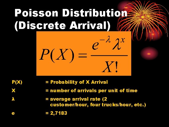
Poisson Distribution (Discrete Arrival) P(X) = Probability of X Arrival X = number of arrivals per unit of time λ = average arrival rate (2 customer/hour, four trucks/hour, etc. ) e = 2, 7183

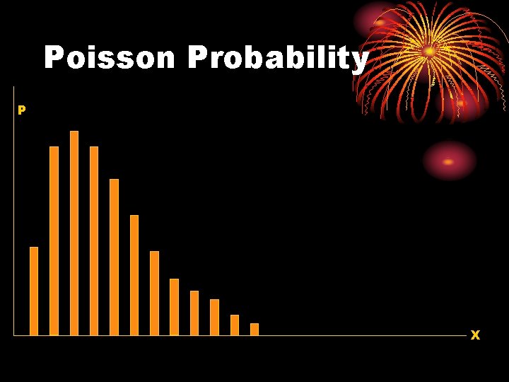
Poisson Probability P X

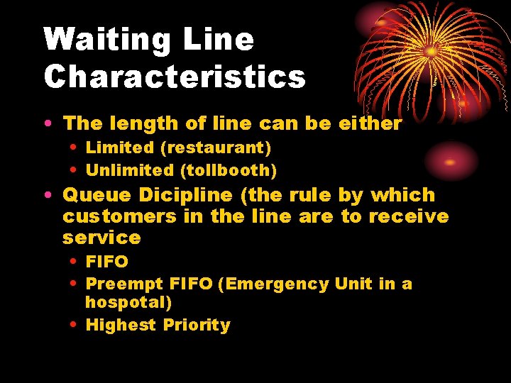
Waiting Line Characteristics • The length of line can be either • Limited (restaurant) • Unlimited (tollbooth) • Queue Dicipline (the rule by which customers in the line are to receive service • FIFO • Preempt FIFO (Emergency Unit in a hospotal) • Highest Priority

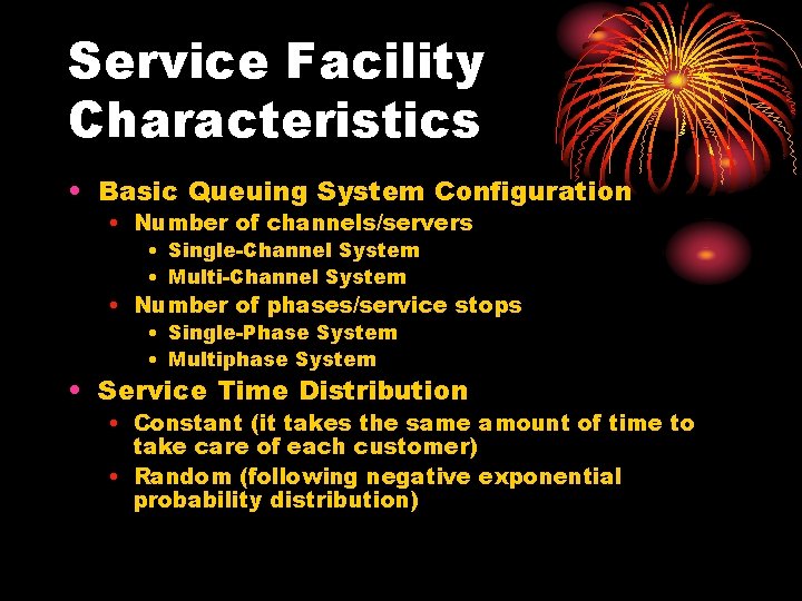
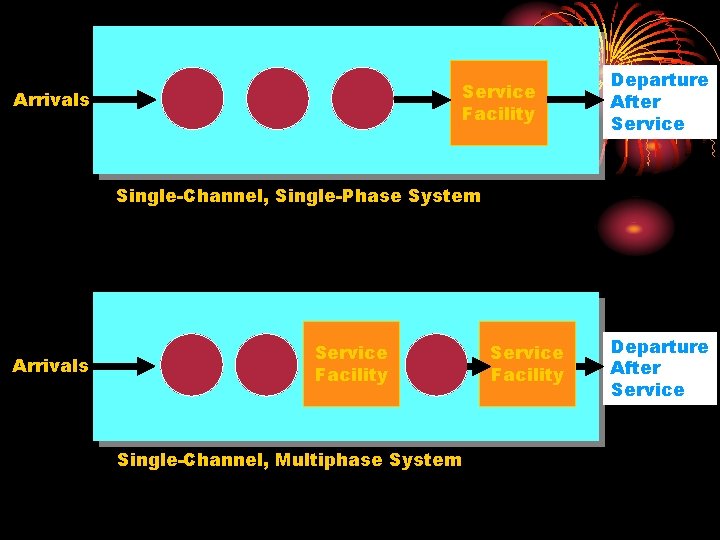
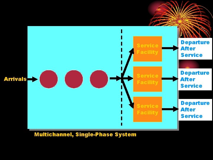
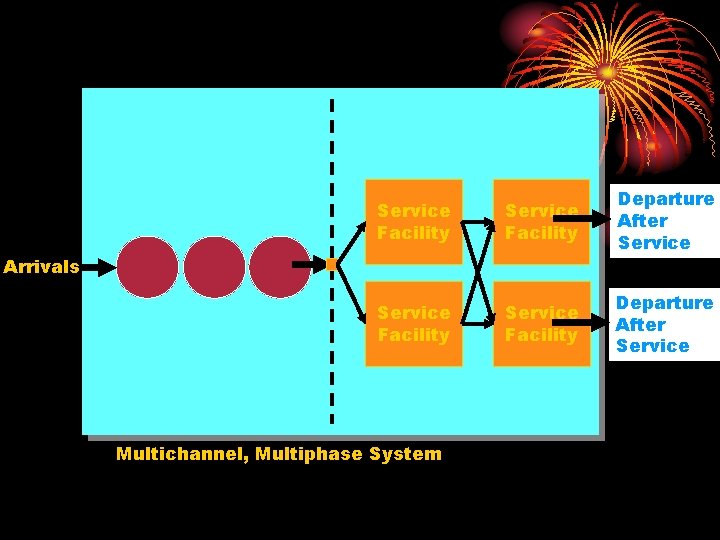
Service Facility Characteristics • Basic Queuing System Configuration • Number of channels/servers • Single-Channel System • Multi-Channel System • Number of phases/service stops • Single-Phase System • Multiphase System • Service Time Distribution • Constant (it takes the same amount of time to take care of each customer) • Random (following negative exponential probability distribution)

Service Facility Arrivals Departure After Service Single-Channel, Single-Phase System Arrivals Service Facility Single-Channel, Multiphase System Service Facility Departure After Service

Arrivals Multichannel, Single-Phase System Service Facility Departure After Service

Service Facility Departure After Service Arrivals Multichannel, Multiphase System

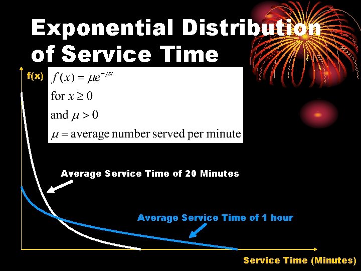
Exponential Distribution of Service Time f(x) Average Service Time of 20 Minutes Average Service Time of 1 hour Service Time (Minutes)

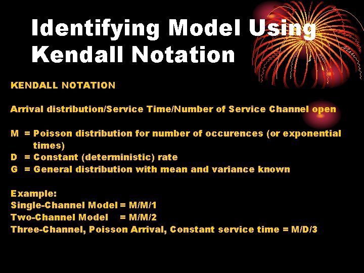
Identifying Model Using Kendall Notation KENDALL NOTATION Arrival distribution/Service Time/Number of Service Channel open M = Poisson distribution for number of occurences (or exponential times) D = Constant (deterministic) rate G = General distribution with mean and variance known Example: Single-Channel Model = M/M/1 Two-Channel Model = M/M/2 Three-Channel, Poisson Arrival, Constant service time = M/D/3

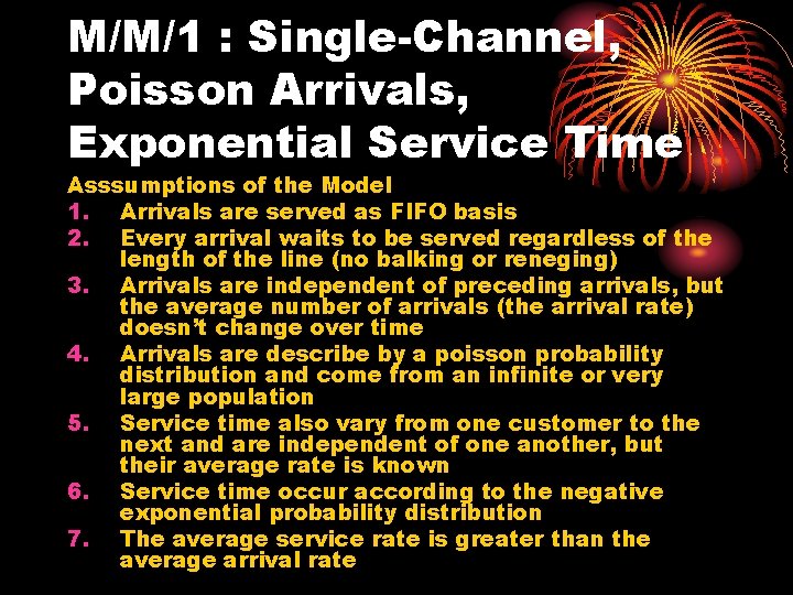
M/M/1 : Single-Channel, Poisson Arrivals, Exponential Service Time Asssumptions of the Model 1. Arrivals are served as FIFO basis 2. Every arrival waits to be served regardless of the length of the line (no balking or reneging) 3. Arrivals are independent of preceding arrivals, but the average number of arrivals (the arrival rate) doesn’t change over time 4. Arrivals are describe by a poisson probability distribution and come from an infinite or very large population 5. Service time also vary from one customer to the next and are independent of one another, but their average rate is known 6. Service time occur according to the negative exponential probability distribution 7. The average service rate is greater than the average arrival rate

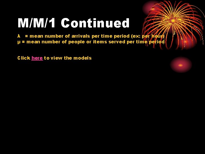
M/M/1 Continued λ = mean number of arrivals per time period (ex: per hour) µ = mean number of people or items served per time period Click here to view the models