Video Shot Detection CIS 581 Course Project Heshan

Video Shot Detection CIS 581 Course Project Heshan Lin

Agenda What’s shot detection? l Classification of shot detection l Close look to hard cuts detection l Experiments and Results l

What’s Shot Detection l l l Problem definition – shot detection: given a video V consisting of n shots, find the beginning and end of each shot. Also known as shot boundary detection or transition detection. It is fundamental to any kind of video analysis and video application since it enables segmentation of a video into its basic components: the shots.

Classification l l Hard cuts: A cut is an instantaneous transition from one scene to the next. There are no transitional frames between 2 shots. Fades: A fade is a gradual transition between a scene and a constant image (fade-out) or between a constant image and a scene (fade-in).

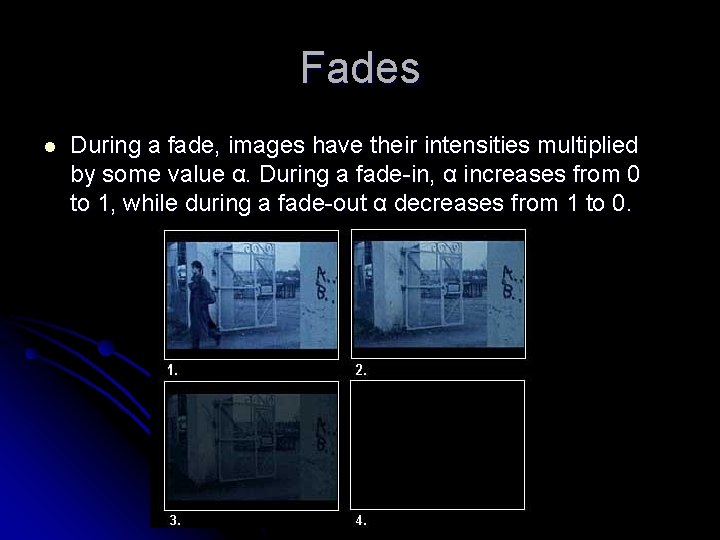
Fades l During a fade, images have their intensities multiplied by some value α. During a fade-in, α increases from 0 to 1, while during a fade-out α decreases from 1 to 0.

Classification l l l Hard cuts: A cut is an instantaneous transition from one scene to the next. Fades: A fade is a gradual transition between a scene and a constant image (fade-out) or between a constant image and a scene (fade-in). Dissolves: A dissolve is a gradual transition from one scene to another, in which the first scene fades out and the second scene fades in.

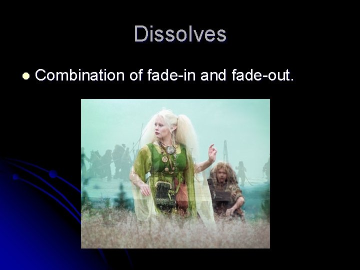
Dissolves l Combination of fade-in and fade-out.

Classification l l Hard cuts: A cut is an instantaneous transition from one scene to the next. Fades: A fade is a gradual transition between a scene and a constant image (fade-out) or between a constant image and a scene (fade-in). Dissolves: A dissolve is a gradual transition from one scene to another, in which the first scene fades out and the second scene fades in. Wipe: another common scene break is a wipe, in which a line moves across the screen, with the new scene appearing behind the line.

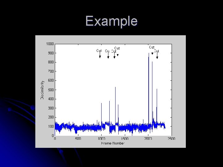
Schema of Cut Detection Calculate a time series of discontinuity feature values f(n) for each frame. Suppose we use function d(x, y) to measure the dissimilarity between frame x and y. The discontinuity feature value for frame n is f(n)=d(n-1, n). l Pick the cuts position from f(n) based on some threshold techniques. l

Example

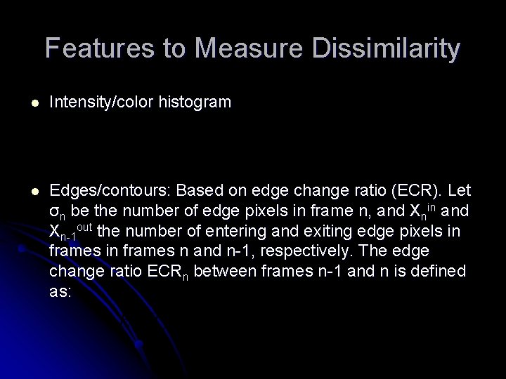
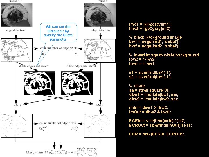
Features to Measure Dissimilarity l Intensity/color histogram l Edges/contours: Based on edge change ratio (ECR). Let σn be the number of edge pixels in frame n, and Xnin and Xn-1 out the number of entering and exiting edge pixels in frames n and n-1, respectively. The edge change ratio ECRn between frames n-1 and n is defined as:

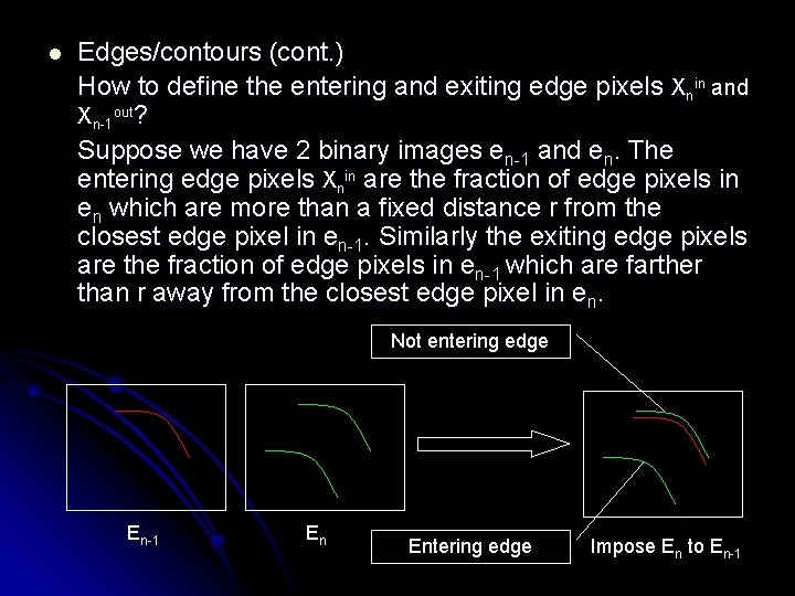
l Edges/contours (cont. ) How to define the entering and exiting edge pixels Xnin and Xn-1 out? Suppose we have 2 binary images en-1 and en. The entering edge pixels Xnin are the fraction of edge pixels in en which are more than a fixed distance r from the closest edge pixel in en-1. Similarly the exiting edge pixels are the fraction of edge pixels in en-1 which are farther than r away from the closest edge pixel in en. Not entering edge En-1 En Entering edge Impose En to En-1

We can set the distance r by specify the Dilate parameter imd 1 = rgb 2 gray(im 1); Imd 2 = rgb 2 gray(im 2); % black background image bw 1 = edge(imd 1, 'sobel'); bw 2 = edge(imd 2, 'sobel'); % invert image to white background ibw 2 = 1 -bw 2; ibw 1 = 1 -bw 1; s 1 = size(find(bw 1), 1); s 2 = size(find(bw 1), 1); % dilate se = strel('square', 3); dbw 1 = imdilate(bw 1, se); dbw 2 = imdilate(bw 2, se); im. In = dbw 1 & ibw 2; im. Out = dbw 2 & ibw 1; ECRIn = size(find(im. In), 1)/s 2; ECROut = size(find(im. Out), 1)/s 1; ECR = max(ECRIn, ECROut);

Thresholding l l Global threshold A hard cut is declared each time the discontinuity value f(n) surpasses a global thresholds. Adaptive threshold A hard cut is detected based on the difference of the current feature values f(n) from its local neighborhood. Generally this kind of method has 2 criteria for a hard cut declaration: - F(n) takes the maximum value inside the neighborhood. - The difference between f(n) and its neighbors’ feature values is bigger than a given threshold.

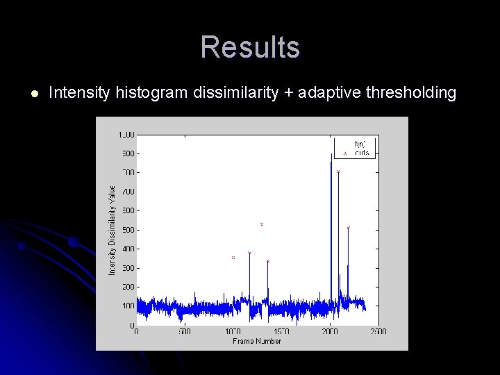
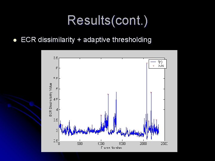
Experiments Input: Mr. Beans movie. (80*112, 2363 frames) l Dissimilarity function - Intensity histogram - Edge change ratio (ECR) l Thresholding - Adaptive threshold based on statistics model. l

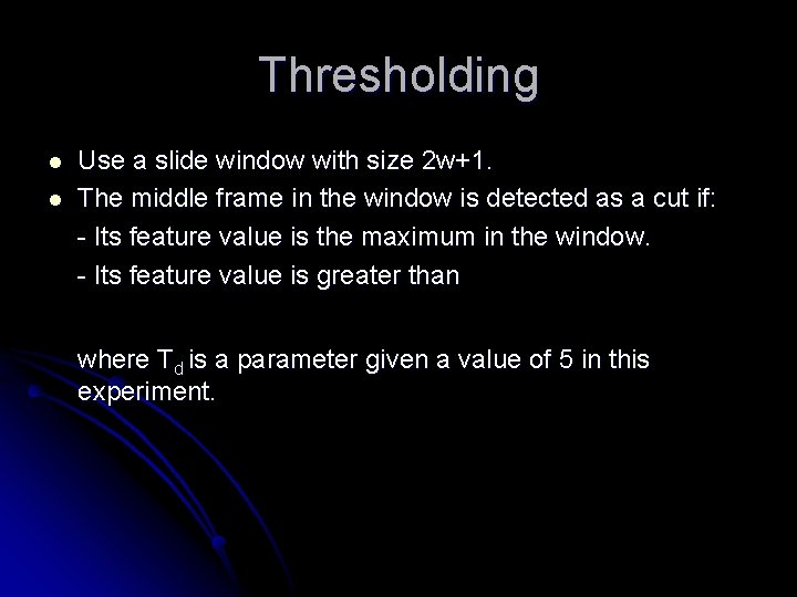
Thresholding l l Use a slide window with size 2 w+1. The middle frame in the window is detected as a cut if: - Its feature value is the maximum in the window. - Its feature value is greater than where Td is a parameter given a value of 5 in this experiment.

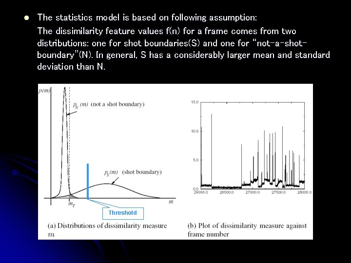
l The statistics model is based on following assumption: The dissimilarity feature values f(n) for a frame comes from two distributions: one for shot boundaries(S) and one for “not-a-shotboundary”(N). In general, S has a considerably larger mean and standard deviation than N. Threshold

Results l Intensity histogram dissimilarity + adaptive thresholding

Results(cont. ) l ECR dissimilarity + adaptive thresholding

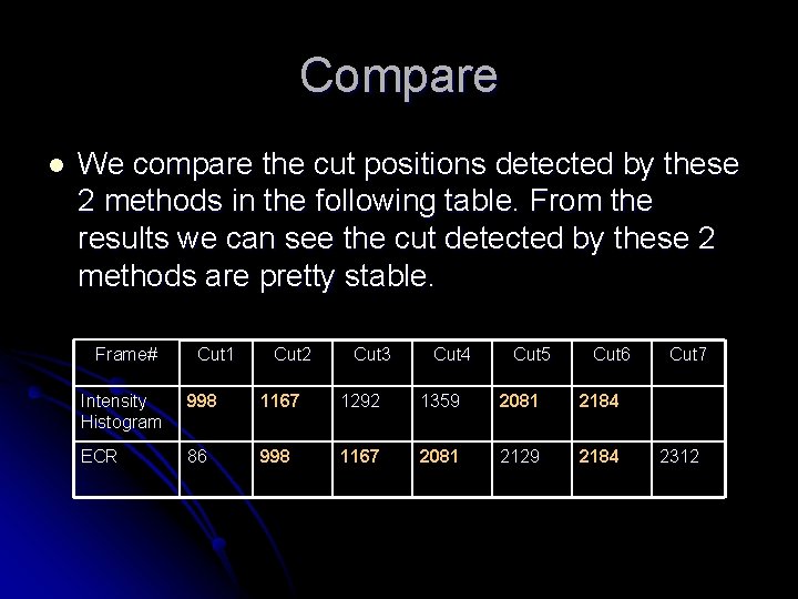
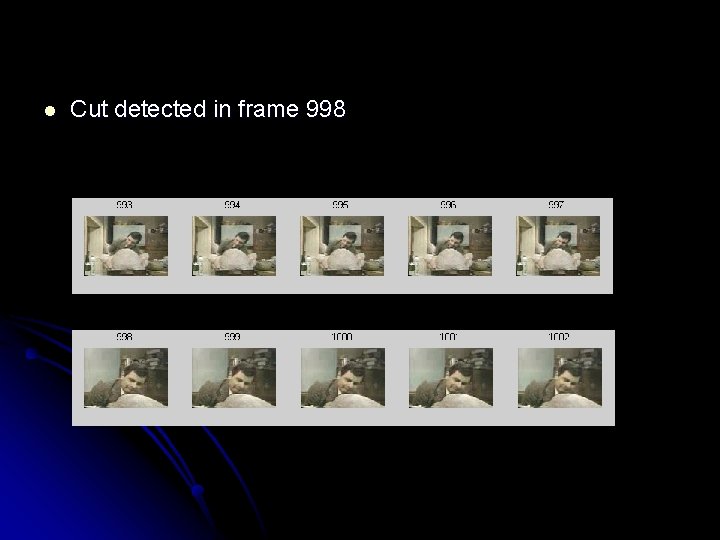
Compare l We compare the cut positions detected by these 2 methods in the following table. From the results we can see the cut detected by these 2 methods are pretty stable. Frame# Cut 1 Cut 2 Cut 3 Cut 4 Cut 5 Cut 6 Intensity Histogram 998 1167 1292 1359 2081 2184 ECR 86 998 1167 2081 2129 2184 Cut 7 2312

l Cut detected in frame 998

Comments