VAR and VEC Using Stata VAR Vector Autoregression

VAR: Vector Autoregression • Assumptions: – – yt: Stationary K-variable vector v: K constant

VAR and VEC • If yt is not stationary, VAR or VEC can only

VEC: Vector Error Correction • If there is no trend in yt, let P

VEC: Vector Error Correction • No-constant or No-drift Model: v = 0 g =

VEC: Vector Error Correction • If there is trend in yt

VEC: Vector Error Correction • No-drift No-trend Model: v = 0, d = 0

Example • • C: Personal Consumption Expenditure Y: Disposable Personal Income C ~ I(1),

Example Johansen Test with trend models and 6 lags • VAR: • VEC: •

Example Johansen Test with constant models and 6 lags • VAR: • VEC: •

Example Johansen Test with constant models and 6 lags • Constant model: v =

Example Johansen Test with trend models and 6 lags • Trend model: d =

Example VEC estimated models with 6 lags • Empirical Model: 1948 q 3 –

VEC Forecasting Estimated Models: 1948 q 3 – 2009 q 4 • No-constant model,

VEC Forecasting Restricted-trend Model, 6 Lags Y = ln(PCE), X = ln(DPI), 2010 q

Slides: 15

Download presentation

VAR and VEC Using Stata

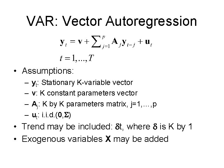
VAR: Vector Autoregression • Assumptions: – – yt: Stationary K-variable vector v: K constant parameters vector Aj: K by K parameters matrix, j=1, …, p ut: i. i. d. (0, S) • Trend may be included: dt, where d is K by 1 • Exogenous variables X may be added

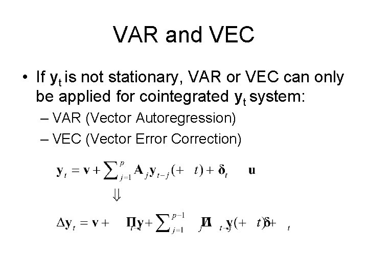
VAR and VEC • If yt is not stationary, VAR or VEC can only be applied for cointegrated yt system: – VAR (Vector Autoregression) – VEC (Vector Error Correction)

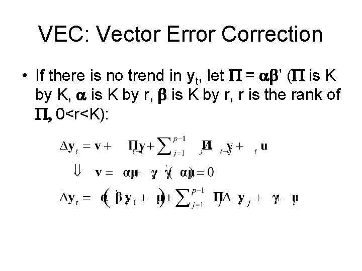
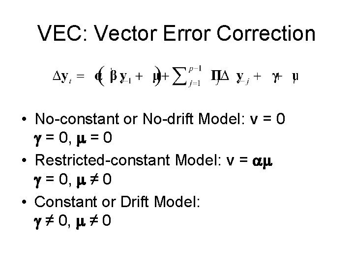
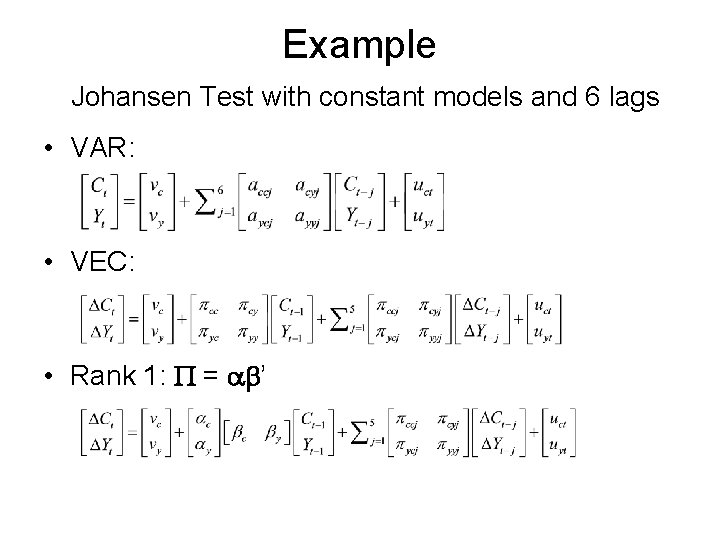
VEC: Vector Error Correction • If there is no trend in yt, let P = ab’ (P is K by K, a is K by r, b is K by r, r is the rank of P, 0<r<K):

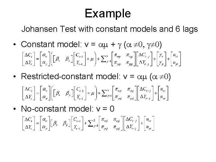
VEC: Vector Error Correction • No-constant or No-drift Model: v = 0 g = 0, m = 0 • Restricted-constant Model: v = am g = 0, m ≠ 0 • Constant or Drift Model: g ≠ 0, m ≠ 0

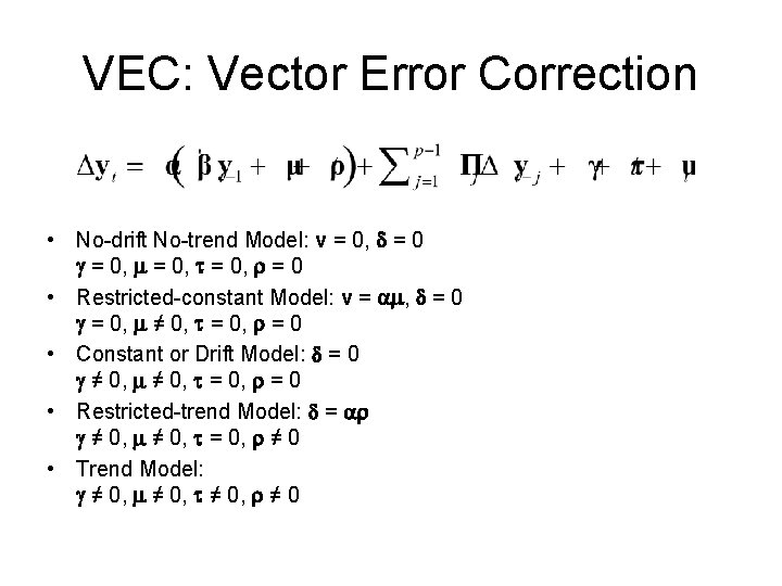
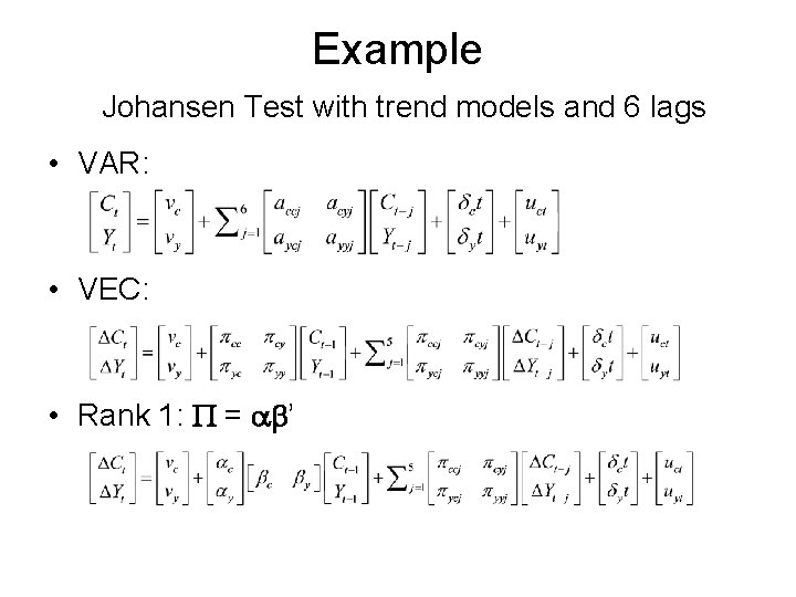
VEC: Vector Error Correction • If there is trend in yt

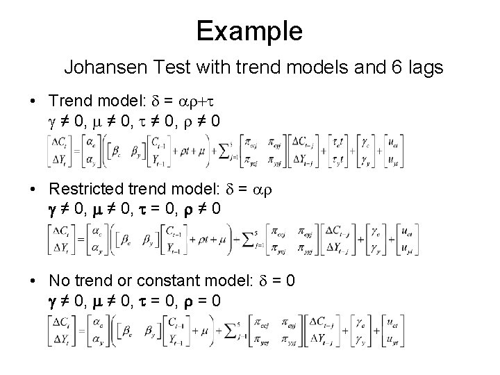
VEC: Vector Error Correction • No-drift No-trend Model: v = 0, d = 0 g = 0, m = 0, t = 0, r = 0 • Restricted-constant Model: v = am, d = 0 g = 0, m ≠ 0, t = 0, r = 0 • Constant or Drift Model: d = 0 g ≠ 0, m ≠ 0, t = 0, r = 0 • Restricted-trend Model: d = ar g ≠ 0, m ≠ 0, t = 0, r ≠ 0 • Trend Model: g ≠ 0, m ≠ 0, t ≠ 0, r ≠ 0

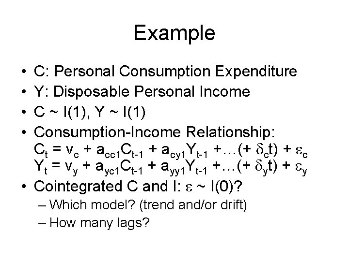
Example • • C: Personal Consumption Expenditure Y: Disposable Personal Income C ~ I(1), Y ~ I(1) Consumption-Income Relationship: Ct = vc + acc 1 Ct-1 + acy 1 Yt-1 +…(+ dct) + ec Yt = vy + ayc 1 Ct-1 + ayy 1 Yt-1 +…(+ dyt) + ey • Cointegrated C and I: e ~ I(0)? – Which model? (trend and/or drift) – How many lags?

Example Johansen Test with trend models and 6 lags • VAR: • VEC: • Rank 1: P = ab’

Example Johansen Test with constant models and 6 lags • VAR: • VEC: • Rank 1: P = ab’

Example Johansen Test with constant models and 6 lags • Constant model: v = am + g (a 0, g 0) • Restricted-constant model: v = am (a 0) • No-constant model: v = 0

Example Johansen Test with trend models and 6 lags • Trend model: d = ar+t g ≠ 0, m ≠ 0, t ≠ 0, r ≠ 0 • Restricted trend model: d = ar g ≠ 0, m ≠ 0, t = 0, r ≠ 0 • No trend or constant model: d = 0 g ≠ 0, m ≠ 0, t = 0, r = 0

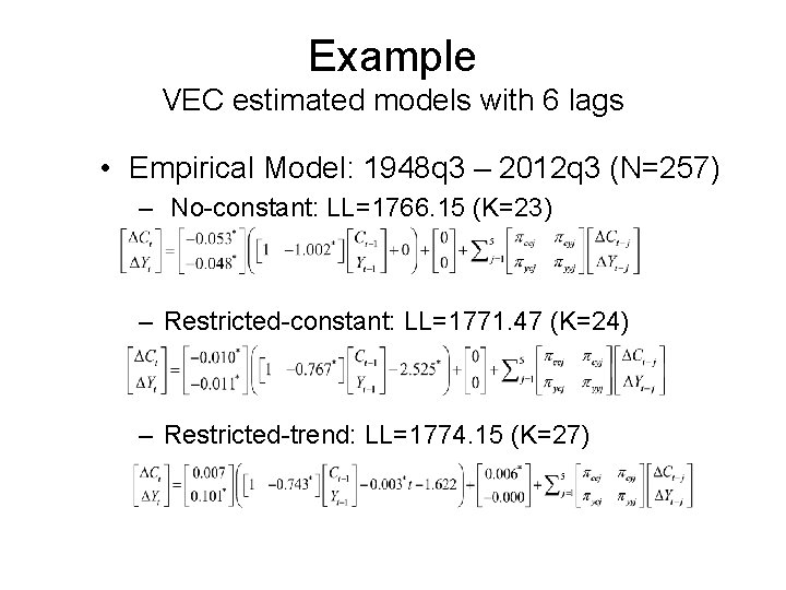
Example VEC estimated models with 6 lags • Empirical Model: 1948 q 3 – 2012 q 3 (N=257) – No-constant: LL=1766. 15 (K=23) – Restricted-constant: LL=1771. 47 (K=24) – Restricted-trend: LL=1774. 15 (K=27)

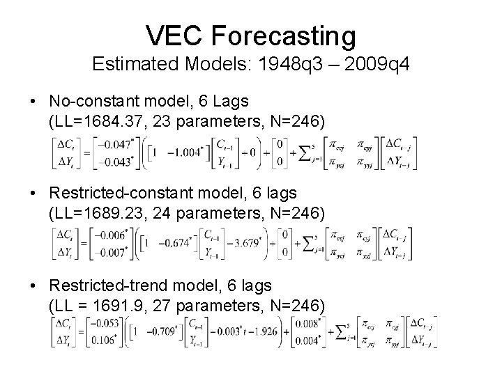
VEC Forecasting Estimated Models: 1948 q 3 – 2009 q 4 • No-constant model, 6 Lags (LL=1684. 37, 23 parameters, N=246) • Restricted-constant model, 6 lags (LL=1689. 23, 24 parameters, N=246) • Restricted-trend model, 6 lags (LL = 1691. 9, 27 parameters, N=246)

VEC Forecasting Restricted-trend Model, 6 Lags Y = ln(PCE), X = ln(DPI), 2010 q 1 -