The Price Elasticities of Demand Supply Chapter 18

The Price Elasticities of Demand Supply Chapter 18 Mc. Graw-Hill/Irwin Copyright © 2011 by The Mc. Graw-Hill Companies, Inc. All rights reserved.

Learning Objectives v After this chapter, you should be able to: 1. 2. 3. 4. 5. 6. 7. Interpret and calculate the elasticity of demand. List and discuss the determinants of elasticity. Examine the relationship between elasticity and total revenue. Define and examine income elasticity of demand cross elasticity of demand. Discuss the elasticity of supply. Name and discuss the three phases of the elasticity of supply over time. Analyze and measure tax incidence. 18 -2

Price Elasticity of Demand The elasticity of demand for a good or service measures the change in quantity demanded in response to a change in price. q In other words, the sensitivity (measured in percentage change) of Qd because of a change (percentage) in P. When P goes up, we know that Qd declines… § but by how much? Elasticity provides us a way of measuring this response. • • • q We will study the price elasticity of demand in three ways: 1. 2. 3. Conceptually (in English) Mathematically (a number) Graphically 18 -3

A Question for Thought and Discussion (Elasticity Conceptually) q Think of two different products and write them down: 1. One in which you are highly price sensitive. For example, you are always checking prices to see when it goes on sale. You will not buy it at any price. 2. Another in which you are not price sensitive. You need this product on a regular basis. You may be loyal to a particular brand. If the price increases, you are likely to buy it anyway. 18 -4

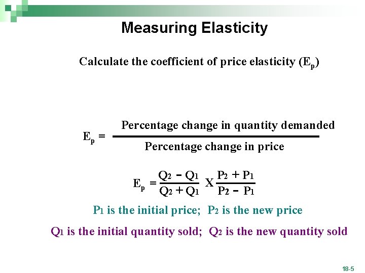
Measuring Elasticity Calculate the coefficient of price elasticity (Ep) Ep = Percentage change in quantity demanded Percentage change in price Q 2 - Q 1 P 2 + P 1 X Ep = Q 2 + Q 1 P 2 - P 1 is the initial price; P 2 is the new price Q 1 is the initial quantity sold; Q 2 is the new quantity sold 18 -5

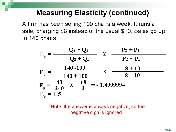
Measuring Elasticity (continued) A firm has been selling 100 chairs a week. It runs a sale, charging $8 instead of the usual $10. Sales go up to 140 chairs. Ep = Q 2 - Q 1 Q 2 + Q 1 X P 2 + P 1 P 2 - P 1 140 -100 8 + 10 X Ep = 8 - 10 140 + 100 40 18 Ep = 240 X -2 = - 1. 4999994 Ep = 1. 5 *Note: the answer is always negative, so the negative sign is ignored. 18 -6

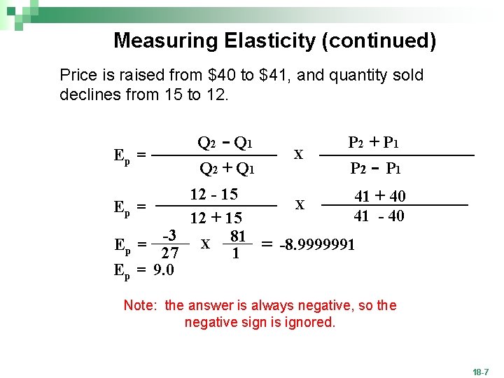
Measuring Elasticity (continued) Price is raised from $40 to $41, and quantity sold declines from 15 to 12. Ep = Q 2 - Q 1 Q 2 + Q 1 X P 2 + P 1 P 2 - P 1 12 - 15 41 + 40 X Ep = 41 - 40 12 + 15 -3 Ep = 27 X 81 1 = -8. 9999991 Ep = 9. 0 Note: the answer is always negative, so the negative sign is ignored. 18 -7

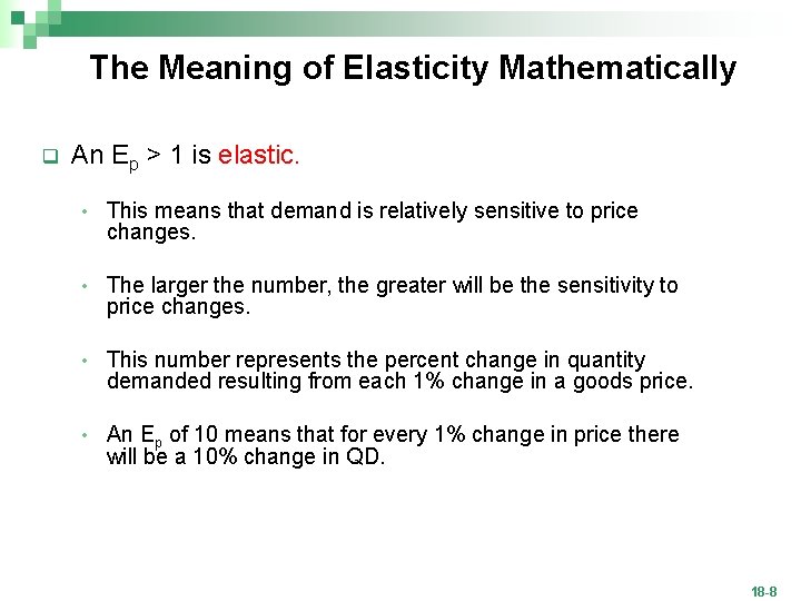
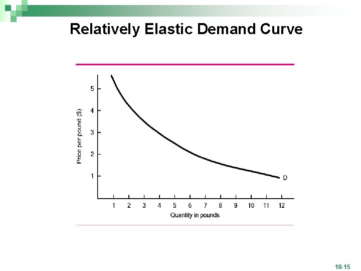
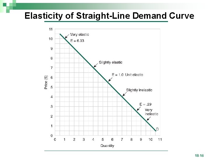
The Meaning of Elasticity Mathematically q An Ep > 1 is elastic. • This means that demand is relatively sensitive to price changes. • The larger the number, the greater will be the sensitivity to price changes. • This number represents the percent change in quantity demanded resulting from each 1% change in a goods price. • An Ep of 10 means that for every 1% change in price there will be a 10% change in QD. 18 -8

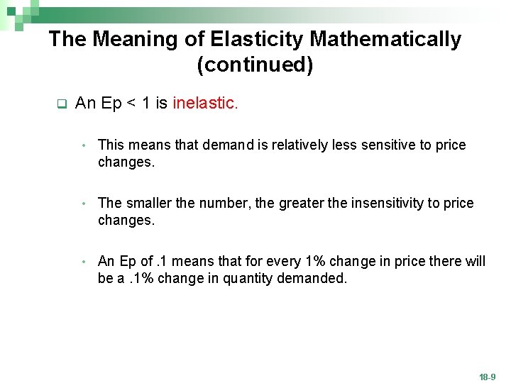
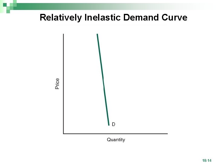
The Meaning of Elasticity Mathematically (continued) q An Ep < 1 is inelastic. • This means that demand is relatively less sensitive to price changes. • The smaller the number, the greater the insensitivity to price changes. • An Ep of. 1 means that for every 1% change in price there will be a. 1% change in quantity demanded. 18 -9

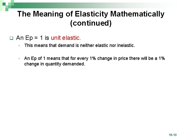
The Meaning of Elasticity Mathematically (continued) q An Ep = 1 is unit elastic. • This means that demand is neither elastic nor inelastic. • An Ep of 1 means that for every 1% change in price there will be a 1% change in quantity demanded. 18 -10

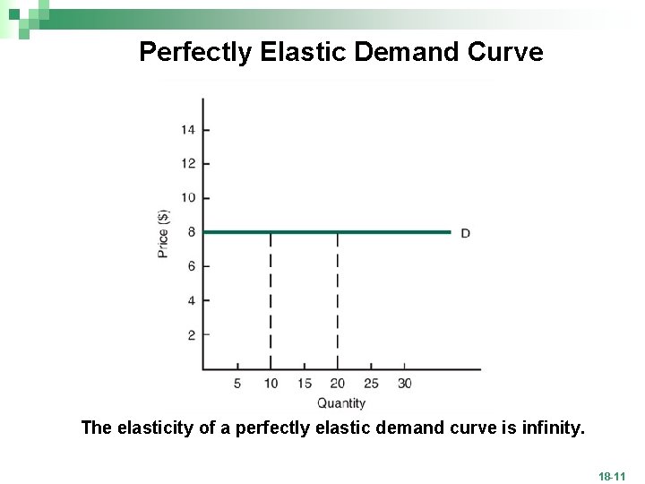
Perfectly Elastic Demand Curve The elasticity of a perfectly elastic demand curve is infinity. 18 -11

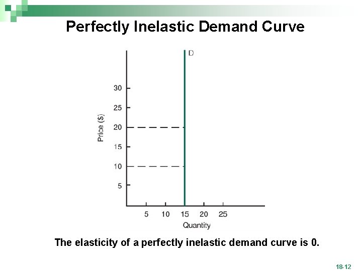
Perfectly Inelastic Demand Curve The elasticity of a perfectly inelastic demand curve is 0. 18 -12

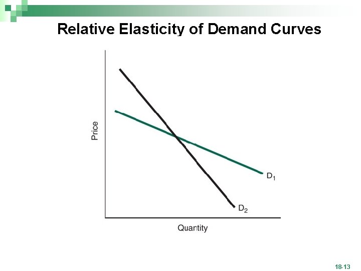
Relative Elasticity of Demand Curves 18 -13

Relatively Inelastic Demand Curve 18 -14

Relatively Elastic Demand Curve 18 -15

Elasticity of Straight-Line Demand Curve 18 -16

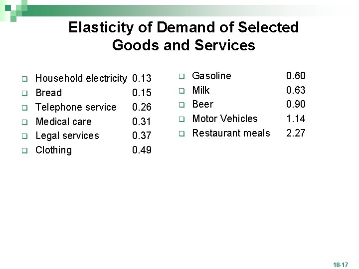
Elasticity of Demand of Selected Goods and Services q q q Household electricity Bread Telephone service Medical care Legal services Clothing 0. 13 0. 15 0. 26 0. 31 0. 37 0. 49 q q q Gasoline Milk Beer Motor Vehicles Restaurant meals 0. 60 0. 63 0. 90 1. 14 2. 27 18 -17

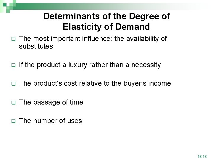
Determinants of the Degree of Elasticity of Demand q The most important influence: the availability of substitutes q If the product a luxury rather than a necessity q The product’s cost relative to the buyer’s income q The passage of time q The number of uses 18 -18

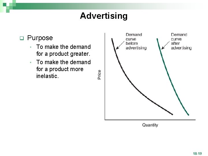
Advertising q Purpose To make the demand for a product greater. • To make the demand for a product more inelastic. • 18 -19

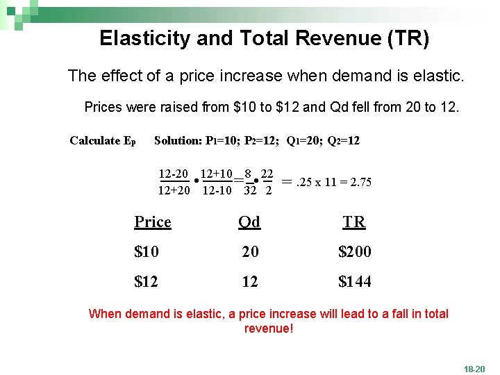
Elasticity and Total Revenue (TR) The effect of a price increase when demand is elastic. Prices were raised from $10 to $12 and Qd fell from 20 to 12. Calculate Ep Solution: P 1=10; P 2=12; Q 1=20; Q 2=12 . . 12 -20 12+10 8 22 = 12+20 12 -10 32 2 = . 25 x 11 = 2. 75 Price Qd TR $10 20 $200 $12 12 $144 When demand is elastic, a price increase will lead to a fall in total revenue! 18 -20

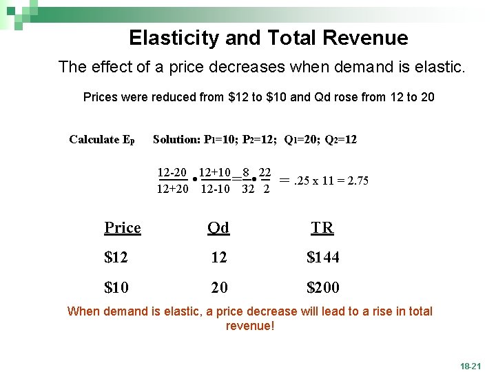
Elasticity and Total Revenue The effect of a price decreases when demand is elastic. Prices were reduced from $12 to $10 and Qd rose from 12 to 20 Calculate Ep Solution: P 1=10; P 2=12; Q 1=20; Q 2=12 . . 12 -20 12+10 8 22 = 12+20 12 -10 32 2 = . 25 x 11 = 2. 75 Price Qd TR $12 12 $144 $10 20 $200 When demand is elastic, a price decrease will lead to a rise in total revenue! 18 -21

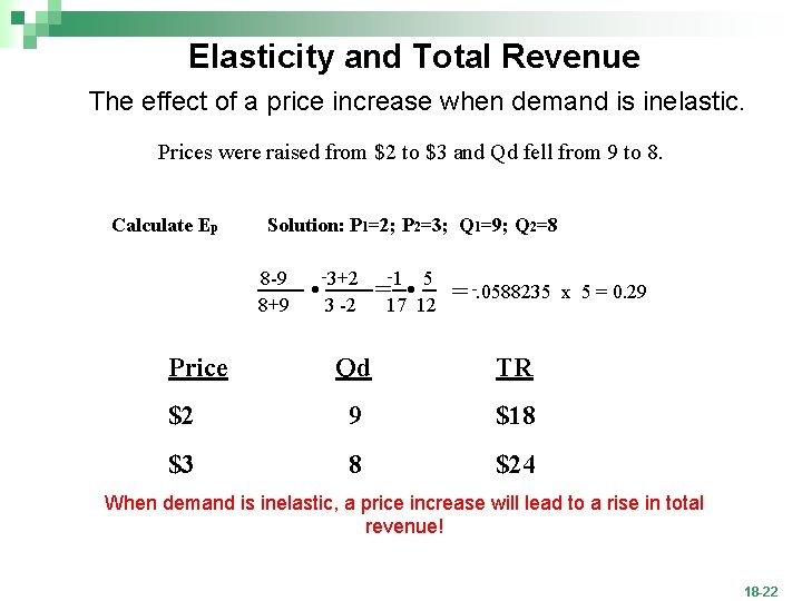
Elasticity and Total Revenue The effect of a price increase when demand is inelastic. Prices were raised from $2 to $3 and Qd fell from 9 to 8. Calculate Ep Solution: P 1=2; P 2=3; Q 1=9; Q 2=8 8 -9 8+9 Price . 33+2 -2 - -1 . 125 =17 = -. 0588235 Qd TR $2 9 $18 $3 8 $24 x 5 = 0. 29 When demand is inelastic, a price increase will lead to a rise in total revenue! 18 -22

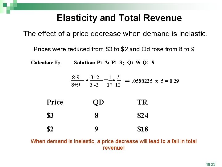
Elasticity and Total Revenue The effect of a price decrease when demand is inelastic. Prices were reduced from $3 to $2 and Qd rose from 8 to 9 Calculate Ep Solution: P 1=2; P 2=3; Q 1=9; Q 2=8 8 -9 8+9 . 33+2 -2 1 . 125 =17 = . 0588235 x 5 = 0. 29 Price QD TR $3 8 $24 $2 9 $18 When demand is inelastic, a price decrease will lead to a fall in total revenue! 18 -23

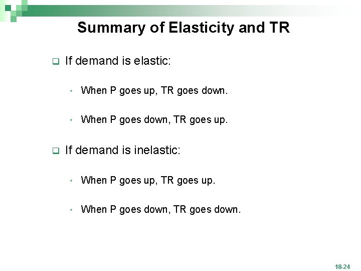
Summary of Elasticity and TR q q If demand is elastic: • When P goes up, TR goes down. • When P goes down, TR goes up. If demand is inelastic: • When P goes up, TR goes up. • When P goes down, TR goes down. 18 -24

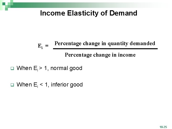
Income Elasticity of Demand Ei = Percentage change in quantity demanded Percentage change in income q When Ei > 1, normal good q When Ei < 1, inferior good 18 -25

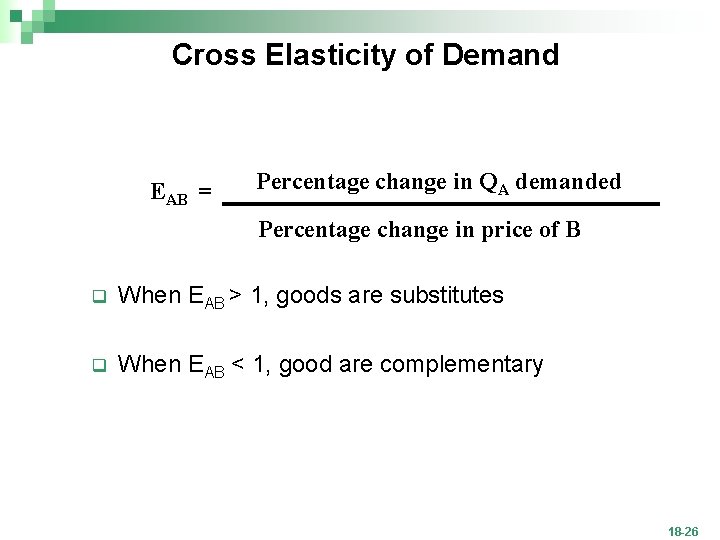
Cross Elasticity of Demand EAB = Percentage change in QA demanded Percentage change in price of B q When EAB > 1, goods are substitutes q When EAB < 1, good are complementary 18 -26

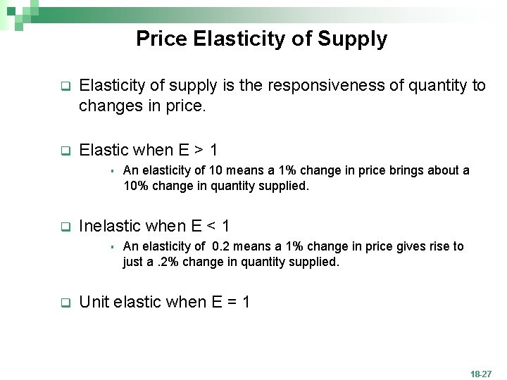
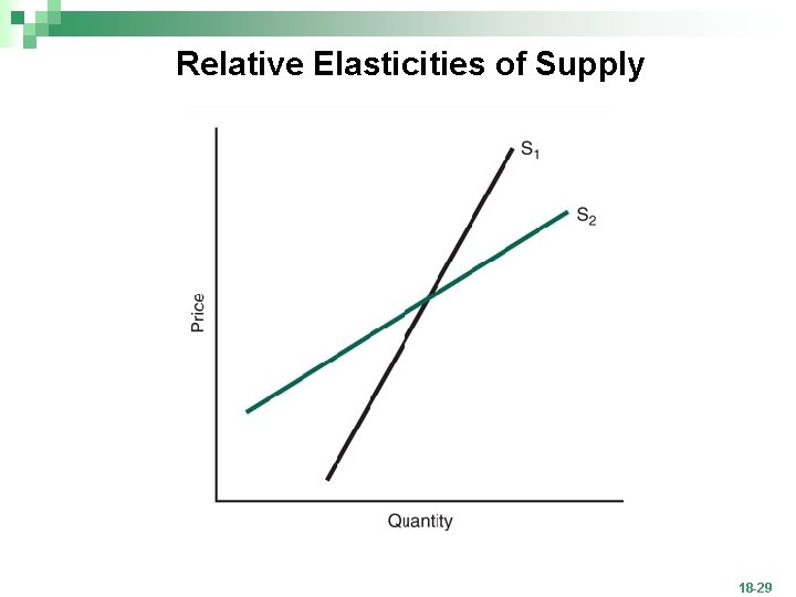
Price Elasticity of Supply q Elasticity of supply is the responsiveness of quantity to changes in price. q Elastic when E > 1 § q Inelastic when E < 1 § q An elasticity of 10 means a 1% change in price brings about a 10% change in quantity supplied. An elasticity of 0. 2 means a 1% change in price gives rise to just a. 2% change in quantity supplied. Unit elastic when E = 1 18 -27

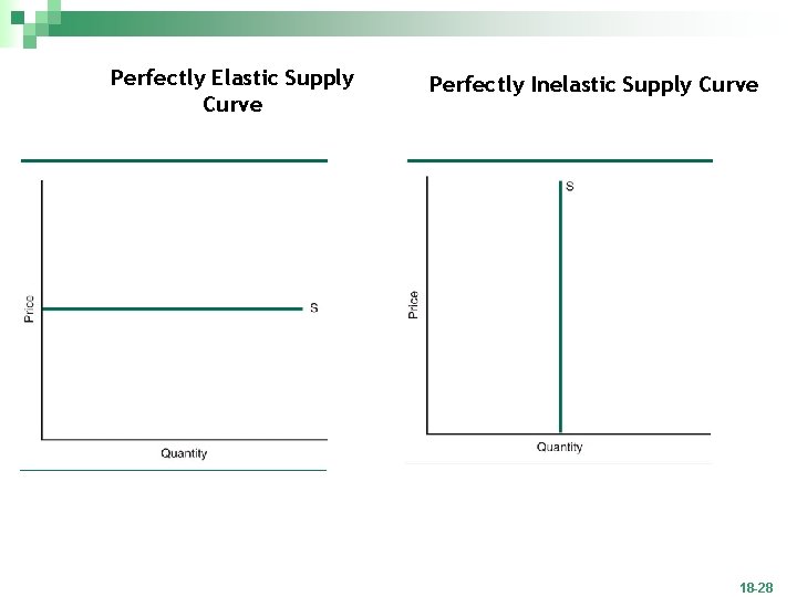
Perfectly Elastic Supply Curve Perfectly Inelastic Supply Curve 18 -28

Relative Elasticities of Supply 18 -29

Elasticity Over Time q Supply grows more elastic over time, especially when enough time has passed for new firm’s to enter the industry and for existing firms to increase their output. q Economists have identified three distinct time periods: 1. 2. 3. The market period The short run The long run 18 -30

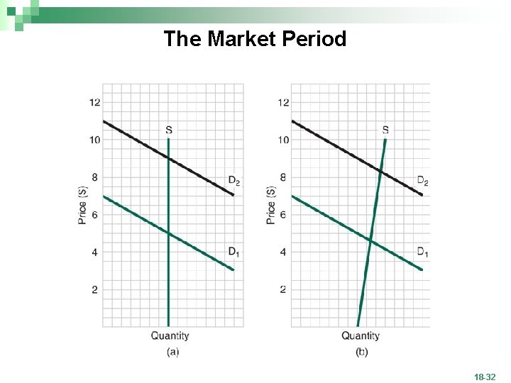
The Market Period q Market period: The time immediately after a change in market price during which the sellers can’t respond by changing the quantity supplied. • During this period the supply curve may be perfectly inelastic or with some positive slope because firms have limited ability to increase output. 18 -31

The Market Period 18 -32

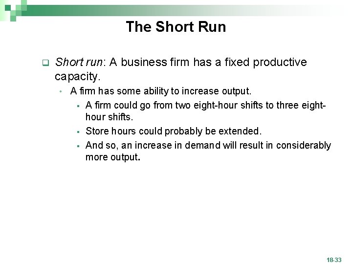
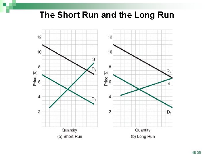
The Short Run q Short run: A business firm has a fixed productive capacity. • A firm has some ability to increase output. § A firm could go from two eight-hour shifts to three eighthour shifts. § Store hours could probably be extended. § And so, an increase in demand will result in considerably more output. 18 -33

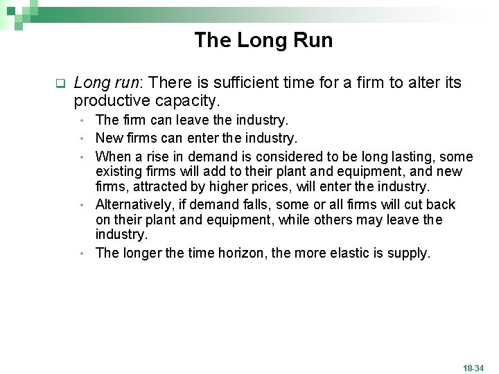
The Long Run q Long run: There is sufficient time for a firm to alter its productive capacity. • • • The firm can leave the industry. New firms can enter the industry. When a rise in demand is considered to be long lasting, some existing firms will add to their plant and equipment, and new firms, attracted by higher prices, will enter the industry. Alternatively, if demand falls, some or all firms will cut back on their plant and equipment, while others may leave the industry. The longer the time horizon, the more elastic is supply. 18 -34

The Short Run and the Long Run 18 -35

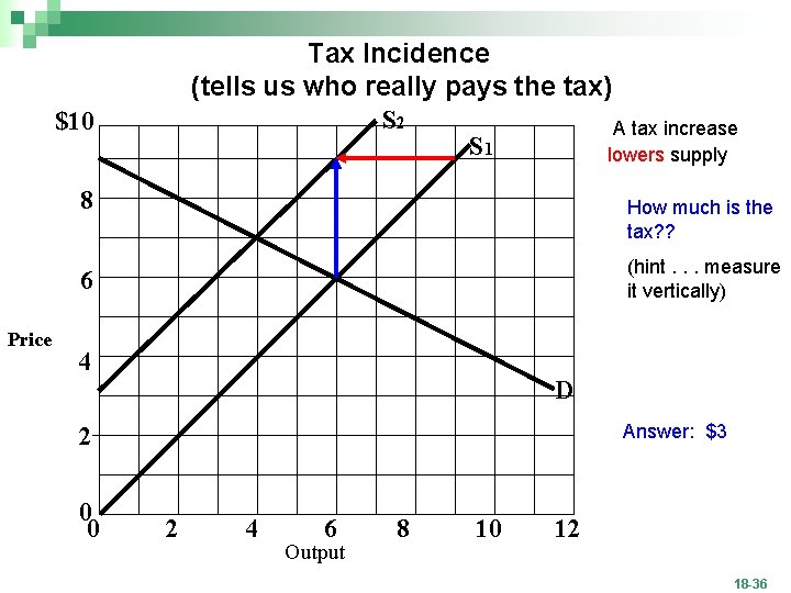
Tax Incidence (tells us who really pays the tax) S 2 A tax increase S 1 lowers supply $10 8 How much is the tax? ? (hint. . . measure it vertically) 6 Price 4 D Answer: $3 2 0 0 2 4 6 Output 8 10 12 18 -36

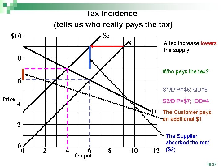
Tax Incidence (tells us who really pays the tax) S 2 A tax increase lowers S 1 $10 the supply. 8 Who pays the tax? 6 S 1/D P=$6; QD=6 Price S 2/D P=$7; QD=4 4 D 2 0 0 2 4 6 Output 8 10 12 The Customer pays an additional $1 The Supplier absorbed the rest ($2) 18 -37

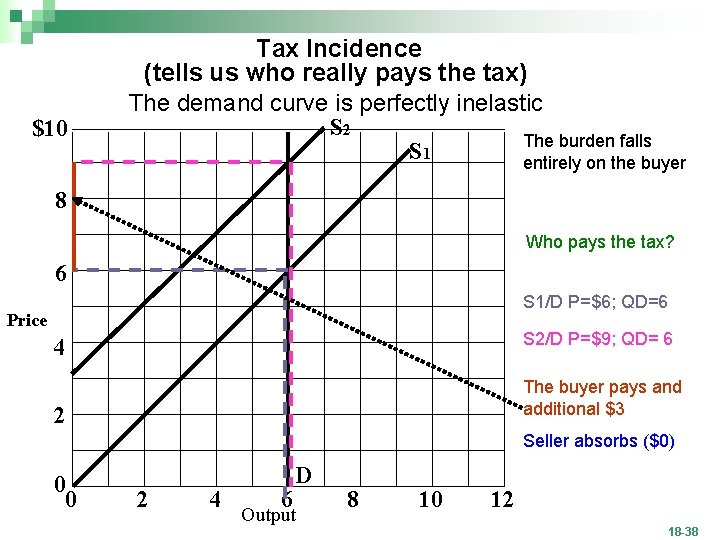
$10 Tax Incidence (tells us who really pays the tax) The demand curve is perfectly inelastic S 2 The burden falls S 1 entirely on the buyer 8 Who pays the tax? 6 S 1/D P=$6; QD=6 Price S 2/D P=$9; QD= 6 4 The buyer pays and additional $3 2 Seller absorbs ($0) 0 0 2 4 6 D Output 8 10 12 18 -38

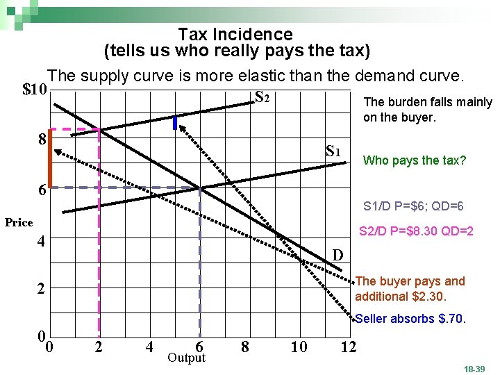
Tax Incidence (tells us who really pays the tax) The supply curve is more elastic than the demand curve. $10 S 2 The burden falls mainly on the buyer. 8 S 1 Who pays the tax? 6 S 1/D P=$6; QD=6 Price S 2/D P=$8. 30 QD=2 4 D The buyer pays and additional $2. 30. 2 Seller absorbs $. 70. 0 0 2 4 6 Output 8 10 12 18 -39

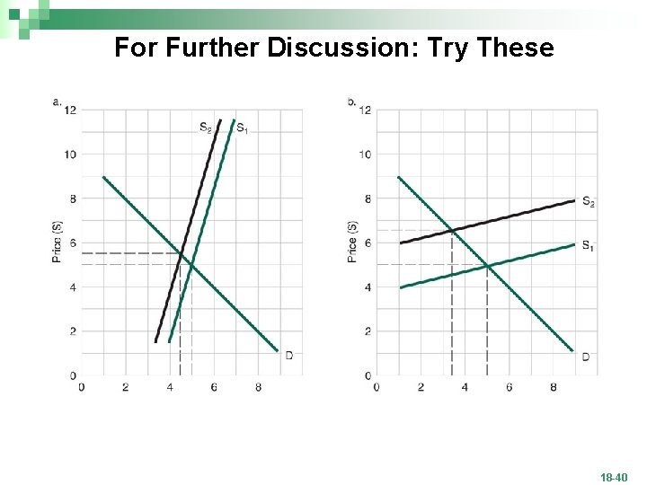
For Further Discussion: Try These 18 -40

Summary of Tax Incidence q When supply is perfectly inelastic, the seller bears the entire tax burden. q When supply is perfectly elastic, the buyer bears entire tax burden. q As the elasticity of demand rises, the tax burden is shifted from the buyer to the seller. q As the elasticity of supply rises, the tax burden is shifted from the seller to the buyer. 18 -41

Current Issue: Oil and Gasoline q In the short run, demand for oil is inelastic. • • q When gas prices rise most drivers do not drive less. Long run: people tend to buy more fuel efficient cars and demand becomes more elastic. Over time, the supply of oil becomes more elastic. Long run: oil production is increased significantly due to increased oil exploration and increased flows from producing oil fields. • The supply of oil becomes more elastic in the long run. • q The heating oil market is similar. Short run: people do not sell their homes or switch from oil to natural gas when oil prices rise. • Long run: fewer oil furnaces will be installed and perhaps solar panels will be installed. • The demand for heating oil will become more elastic. • 18 -42

Questions for Thought and Discussion: How Elastic is Your Demand for Food? q No matter how low your income, you still have to eat. q If your income went down significantly, you would buy less expensive food. q Higher priced foods become luxuries. q Lower priced foods become necessities. q The bottom line is A good or service is a necessity if its share of your budget falls as your income rises. • It is a luxury if its share of your budget rises as income rises. • 18 -43