Testing Variances Sample variances s 2 and sample

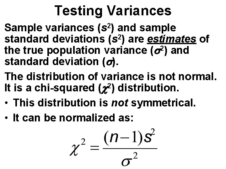
Testing Variances Sample variances (s 2) and sample standard deviations (s 2) are estimates of the true population variance (s 2) and standard deviation (s). The distribution of variance is not normal. It is a chi-squared (c 2) distribution. • This distribution is not symmetrical. • It can be normalized as:

Why Do We Test Variances? In several statistical tests comparing groups, one of the key assumptions is that the variances of the two groups are equal (i. e. , s. A 2 = s. B 2 = s. C 2 = …). In some research tests, the question is not where the means are different, but whether the variances are different. For example: • Although the mean age at attaining puberty is the same, there may be greater variability that age in girls vs. boys. • The average number of eggs in a clutch may be constant, but the percent that hatch may not be.

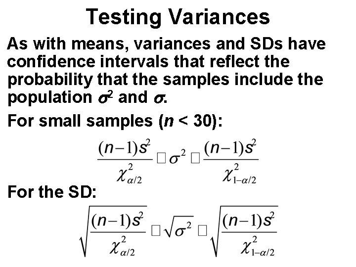
Testing Variances As with means, variances and SDs have confidence intervals that reflect the probability that the samples include the population s 2 and s. For small samples (n < 30): For the SD:

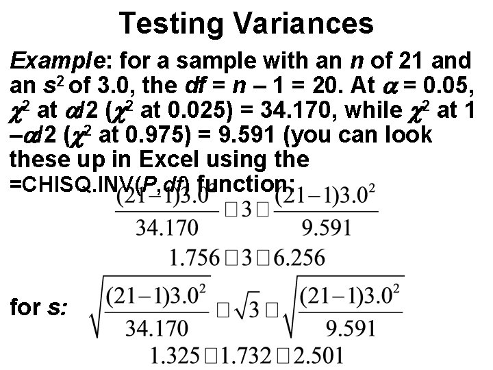
Testing Variances Example: for a sample with an n of 21 and an s 2 of 3. 0, the df = n – 1 = 20. At a = 0. 05, c 2 at a/2 (c 2 at 0. 025) = 34. 170, while c 2 at 1 –a/2 (c 2 at 0. 975) = 9. 591 (you can look these up in Excel using the =CHISQ. INV(P, df) function: for s:

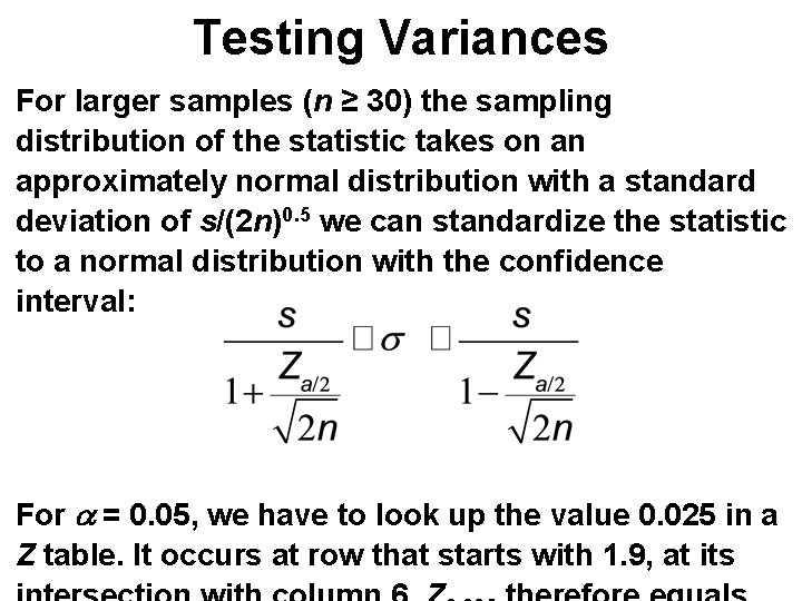
Testing Variances For larger samples (n ≥ 30) the sampling distribution of the statistic takes on an approximately normal distribution with a standard deviation of s/(2 n)0. 5 we can standardize the statistic to a normal distribution with the confidence interval: For a = 0. 05, we have to look up the value 0. 025 in a Z table. It occurs at row that starts with 1. 9, at its

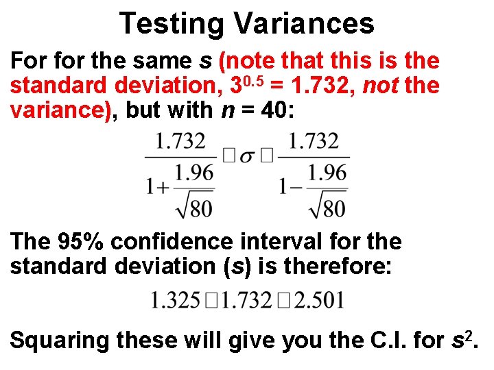
Testing Variances For for the same s (note that this is the standard deviation, 30. 5 = 1. 732, not the variance), but with n = 40: The 95% confidence interval for the standard deviation (s) is therefore: Squaring these will give you the C. I. for s 2.

Comparing Variances to a Hypothetical Value We are often interested in determining how a sample variance is related to a hypothesized value for the population variance (s 2). This involves the same sort of probability statement that we used for the single-sample test of means. In the case of the variance, we use the c 2 distribution for small sample sizes and the Z distribution for large samples. Both small and large sample tests are very dependent on the underlying data being normally distributed.

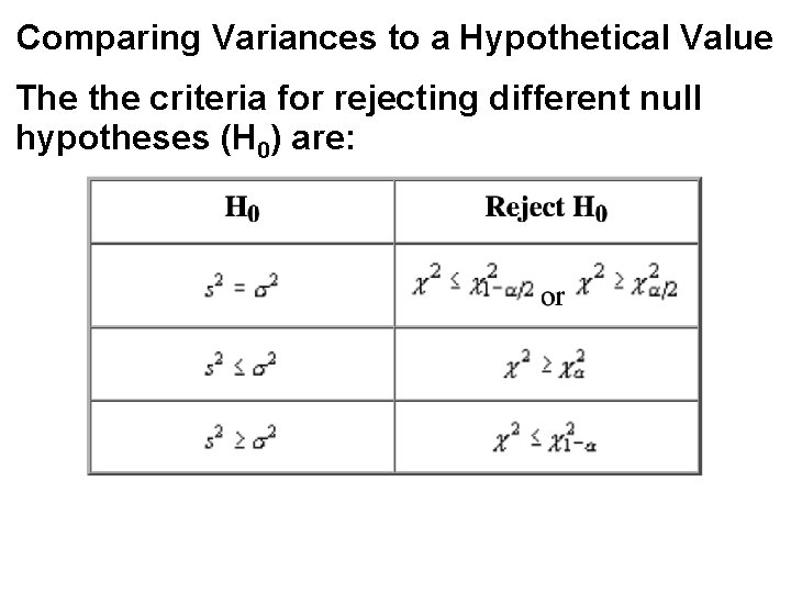
Comparing Variances to a Hypothetical Value The the criteria for rejecting different null hypotheses (H 0) are:

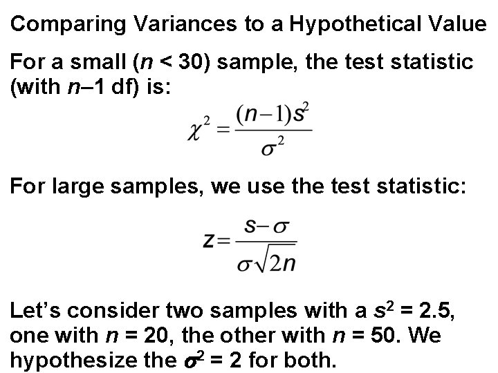
Comparing Variances to a Hypothetical Value For a small (n < 30) sample, the test statistic (with n– 1 df) is: For large samples, we use the test statistic: Let’s consider two samples with a s 2 = 2. 5, one with n = 20, the other with n = 50. We hypothesize the s 2 = 2 for both.

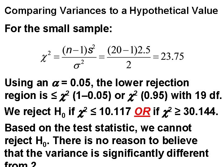
Comparing Variances to a Hypothetical Value For the small sample: Using an a = 0. 05, the lower rejection region is ≤ c 2 (1– 0. 05) or c 2 (0. 95) with 19 df. We reject H 0 if c 2 ≤ 10. 117 OR if c 2 ≥ 30. 144. Based on the test statistic, we cannot reject H 0. There is no reason to believe that the variance is significantly different

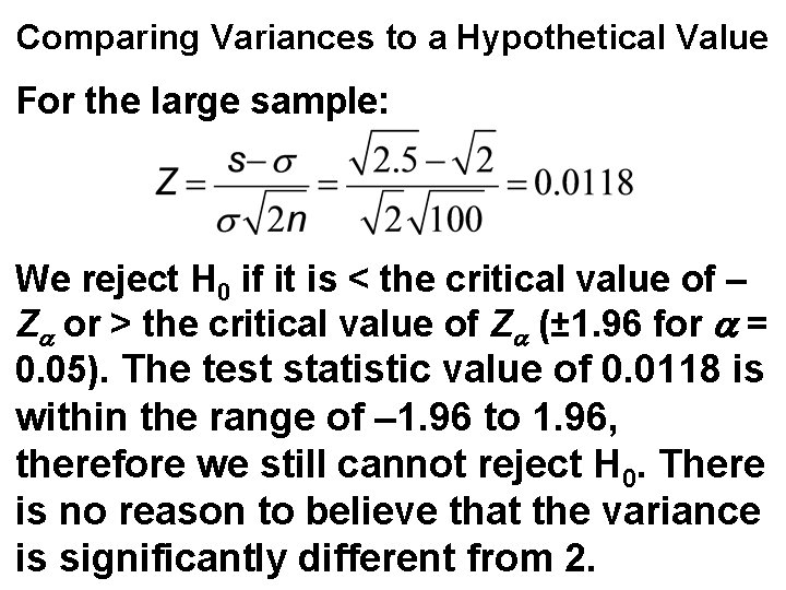
Comparing Variances to a Hypothetical Value For the large sample: We reject H 0 if it is < the critical value of – Za or > the critical value of Za (± 1. 96 for a = 0. 05). The test statistic value of 0. 0118 is within the range of – 1. 96 to 1. 96, therefore we still cannot reject H 0. There is no reason to believe that the variance is significantly different from 2.

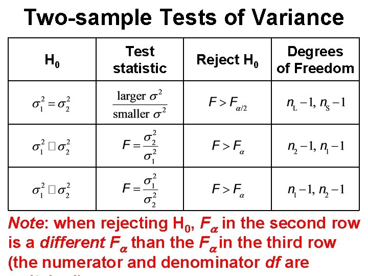
Two-sample Tests of Variance H 0 Test statistic Reject H 0 Degrees of Freedom Note: when rejecting H 0, Fa in the second row is a different Fa than the Fa in the third row (the numerator and denominator df are

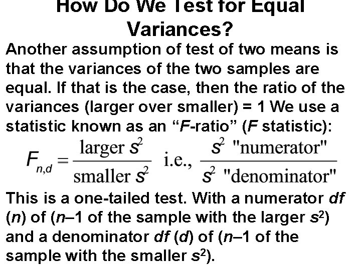
How Do We Test for Equal Variances? Another assumption of test of two means is that the variances of the two samples are equal. If that is the case, then the ratio of the variances (larger over smaller) = 1 We use a statistic known as an “F-ratio” (F statistic): This is a one-tailed test. With a numerator df (n) of (n– 1 of the sample with the larger s 2) and a denominator df (d) of (n– 1 of the sample with the smaller s 2).

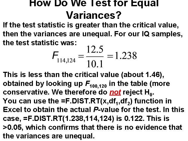
How Do We Test for Equal Variances? If the test statistic is greater than the critical value, then the variances are unequal. For our IQ samples, the test statistic was: This is less than the critical value (about 1. 46), obtained by looking up F 100, 120 in the table (more conservative. We therefore do not reject H 0. You can use the =F. DIST. RT(x, df 1, df 2) function in Excel to obtain the actual P-value for the test. In this case, =F. DIST. RT(1. 238, 114, 124) is 0. 122. This is >0. 05, which confirms that there is no evidence that the variances are unequal.

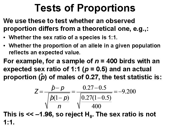
Tests of Proportions We use these to test whether an observed proportion differs from a theoretical one, e. g. , : • Whether the sex ratio of a species is 1: 1. • Whether the proportion of an allele in a given population reflects an expected value. For example, for a sample of n = 400 birds with an expected sex ratio of 1: 1 (p = 0. 5) and an actual ^ proportion (p) of males of 0. 27, the test statistic is: This is << – 1. 96, so reject H 0. The sex ratio is not 1: 1.

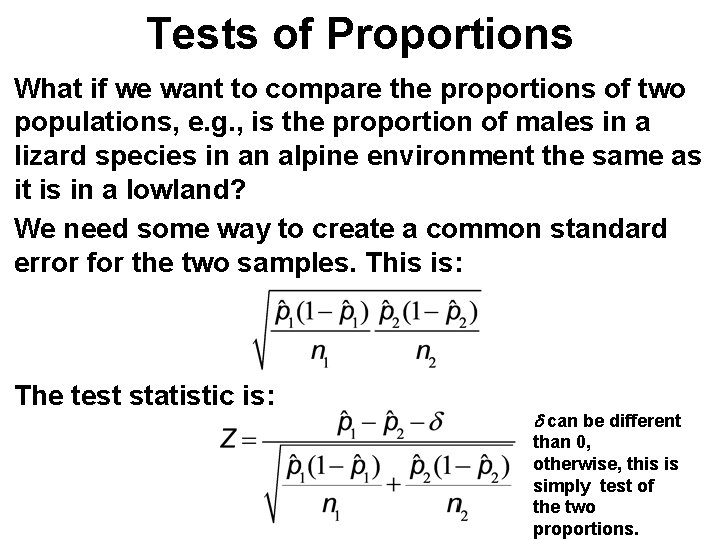
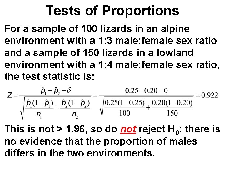
Tests of Proportions What if we want to compare the proportions of two populations, e. g. , is the proportion of males in a lizard species in an alpine environment the same as it is in a lowland? We need some way to create a common standard error for the two samples. This is: The test statistic is: d can be different than 0, otherwise, this is simply test of the two proportions.

Tests of Proportions For a sample of 100 lizards in an alpine environment with a 1: 3 male: female sex ratio and a sample of 150 lizards in a lowland environment with a 1: 4 male: female sex ratio, the test statistic is: This is not > 1. 96, so do not reject H 0: there is no evidence that the proportion of males differs in the two environments.

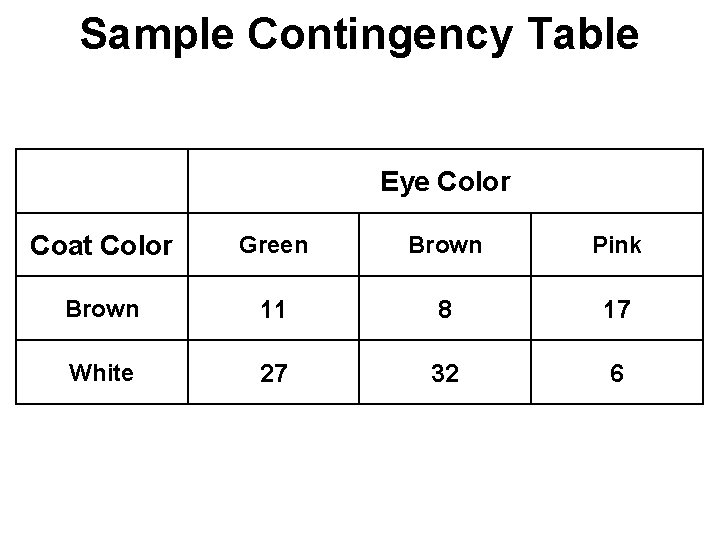
Chi-square (c Tests 2) Tests of proportions have two limitations: • The sample sizes must be large to use the normal approximation to the binomial. • This test is not easily extended to multiple cases. We may be interested in the homogeneity of several proportions. The χ2 test provides a means of achieving this without large sample sizes. In χ2 tests, we produce a table of observations and compare them to expected frequencies. We normally call this an r × c or contingency table.

Sample Contingency Table Eye Color Coat Color Green Brown Pink Brown 11 8 17 White 27 32 6

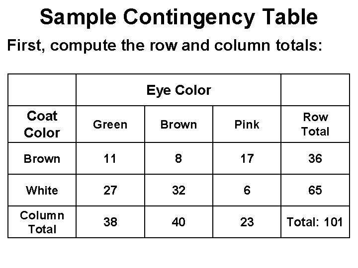
Sample Contingency Table First, compute the row and column totals: Eye Color Coat Color Green Brown Pink Row Total Brown 11 8 17 36 White 27 32 6 65 Column Total 38 40 23 Total: 101

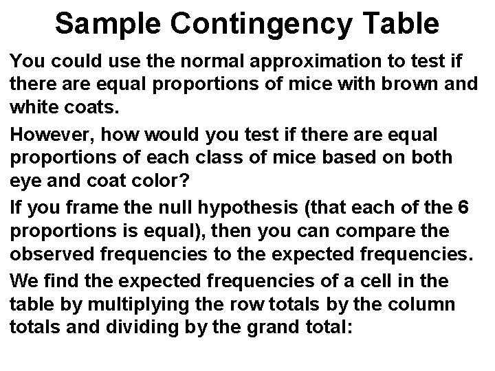
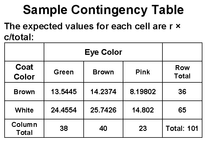
Sample Contingency Table You could use the normal approximation to test if there are equal proportions of mice with brown and white coats. However, how would you test if there are equal proportions of each class of mice based on both eye and coat color? If you frame the null hypothesis (that each of the 6 proportions is equal), then you can compare the observed frequencies to the expected frequencies. We find the expected frequencies of a cell in the table by multiplying the row totals by the column totals and dividing by the grand total:

Sample Contingency Table The expected values for each cell are r × c/total: Eye Color Coat Color Green Brown Pink Row Total Brown 13. 5445 14. 2374 8. 19802 36 White 24. 4554 25. 7426 14. 802 65 Column Total 38 40 23 Total: 101

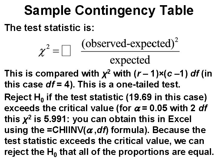
Sample Contingency Table The test statistic is: This is compared with χ2 with (r – 1)×(c – 1) df (in this case df = 4). This is a one-tailed test. Reject H 0 if the test statistic (19. 69 in this case) exceeds the critical value (for a = 0. 05 with 2 df this χ2 is 5. 991: you can obtain this in Excel using the =CHIINV(a , df) formula). Because the test statistic exceeds the critical value, we can reject the H 0 that all of the proportions are equal.

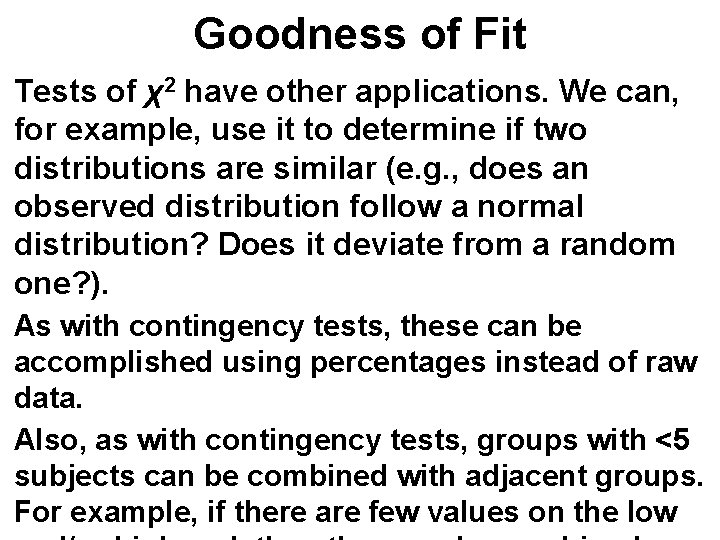
Goodness of Fit Tests of χ2 have other applications. We can, for example, use it to determine if two distributions are similar (e. g. , does an observed distribution follow a normal distribution? Does it deviate from a random one? ). As with contingency tests, these can be accomplished using percentages instead of raw data. Also, as with contingency tests, groups with <5 subjects can be combined with adjacent groups. For example, if there are few values on the low

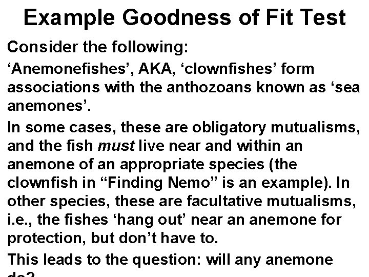
Example Goodness of Fit Test Consider the following: ‘Anemonefishes’, AKA, ‘clownfishes’ form associations with the anthozoans known as ‘sea anemones’. In some cases, these are obligatory mutualisms, and the fish must live near and within an anemone of an appropriate species (the clownfish in “Finding Nemo” is an example). In other species, these are facultative mutualisms, i. e. , the fishes ‘hang out’ near an anemone for protection, but don’t have to. This leads to the question: will any anemone

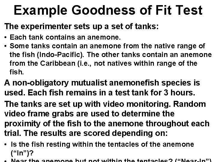
Example Goodness of Fit Test The experimenter sets up a set of tanks: • Each tank contains an anemone. • Some tanks contain an anemone from the native range of the fish (Indo-Pacific). The other tanks contain an anemone from the Caribbean (i. e. , not natives within range of the fish. A non-obligatory mutualist anemonefish species is used. Each fish remains in a test tank for 3 hours. The tanks are set up with video monitoring. Random video frame grabs are used to determine the proximity of the fish to the anemone throughout each trial. The results are scored depending on: • Is the fish resting within the tentacles of the anemone (“In”)?

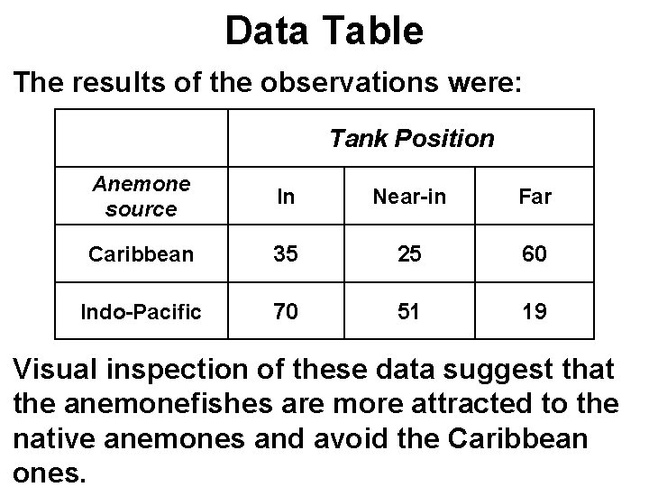
Data Table The results of the observations were: Tank Position Anemone source In Near-in Far Caribbean 35 25 60 Indo-Pacific 70 51 19 Visual inspection of these data suggest that the anemonefishes are more attracted to the native anemones and avoid the Caribbean ones.

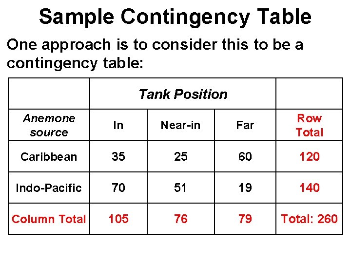
Sample Contingency Table One approach is to consider this to be a contingency table: Tank Position Anemone source In Near-in Far Row Total Caribbean 35 25 60 120 Indo-Pacific 70 51 19 140 Column Total 105 76 79 Total: 260

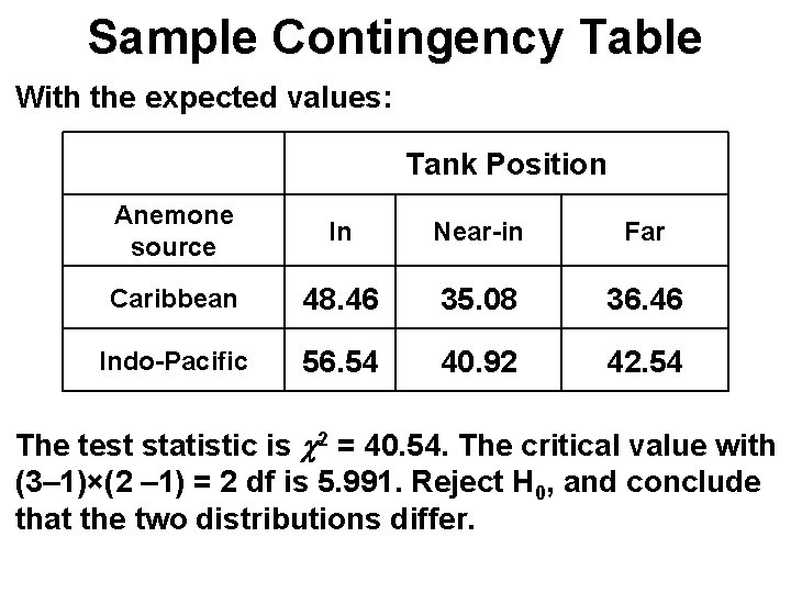
Sample Contingency Table With the expected values: Tank Position Anemone source In Near-in Far Caribbean 48. 46 35. 08 36. 46 Indo-Pacific 56. 54 40. 92 42. 54 The test statistic is c 2 = 40. 54. The critical value with (3– 1)×(2 – 1) = 2 df is 5. 991. Reject H 0, and conclude that the two distributions differ.

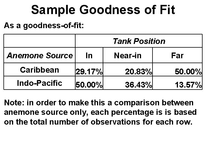
Sample Goodness of Fit As a goodness-of-fit: Tank Position Anemone Source In Near-in Far Caribbean 29. 17% 20. 83% 50. 00% Indo-Pacific 50. 00% 36. 43% 13. 57% Note: in order to make this a comparison between anemone source only, each percentage is is based on the total number of observations for each row.

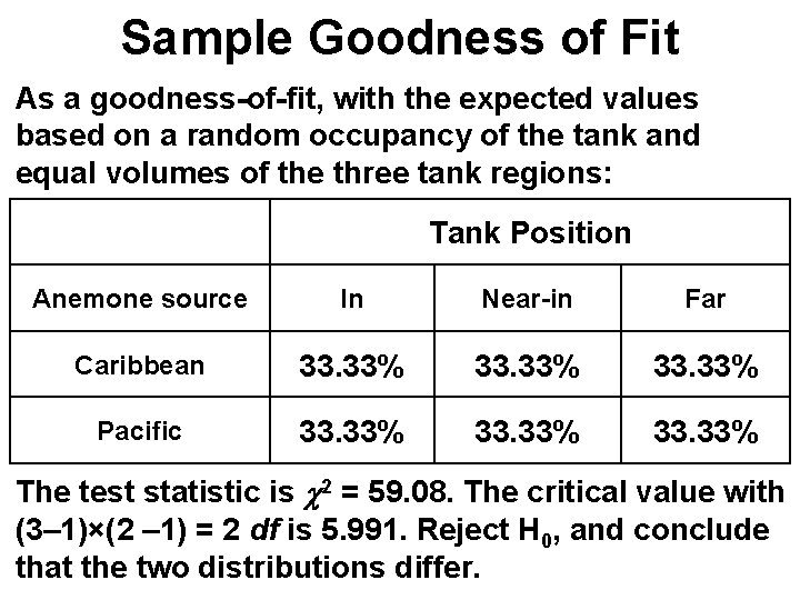
Sample Goodness of Fit As a goodness-of-fit, with the expected values based on a random occupancy of the tank and equal volumes of the three tank regions: Tank Position Anemone source In Near-in Far Caribbean 33. 33% Pacific 33. 33% The test statistic is c 2 = 59. 08. The critical value with (3– 1)×(2 – 1) = 2 df is 5. 991. Reject H 0, and conclude that the two distributions differ.