Statistics cont Psych 231 Research Methods in Psychology

Statistics (cont. ) Psych 231: Research Methods in Psychology

n n Quiz 10 is due on Friday at midnight Class experiment final drafts due in labs this week Announcements

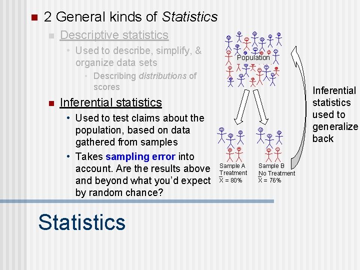
n 2 General kinds of Statistics n Descriptive statistics • Used to describe, simplify, & organize data sets Population • Describing distributions of scores n Inferential statistics used to generalize back Inferential statistics • Used to test claims about the population, based on data gathered from samples • Takes sampling error into account. Are the results above and beyond what you’d expect by random chance? Statistics Sample A Treatment X = 80% Sample B No Treatment X = 76%

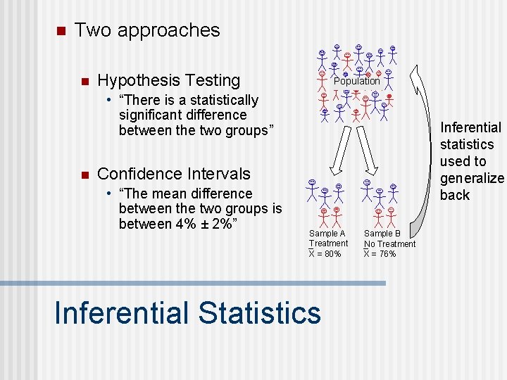
n Two approaches n Hypothesis Testing Population • “There is a statistically significant difference between the two groups” n Inferential statistics used to generalize back Confidence Intervals • “The mean difference between the two groups is between 4% ± 2%” Sample A Treatment X = 80% Inferential Statistics Sample B No Treatment X = 76%

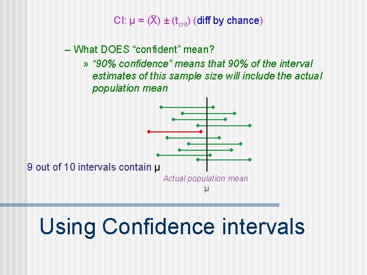
CI: μ = (X) ± (tcrit) (diff by chance) – What DOES “confident” mean? » “ 90% confidence” means that 90% of the interval estimates of this sample size will include the actual population mean 9 out of 10 intervals contain μ Actual population mean μ Using Confidence intervals

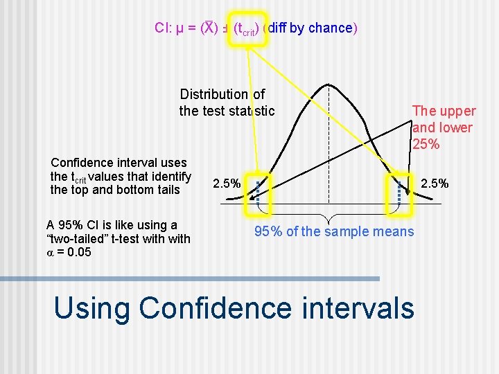
CI: μ = (X) ± (tcrit) (diff by chance) Distribution of the test statistic Confidence interval uses the tcrit values that identify the top and bottom tails A 95% CI is like using a “two-tailed” t-test with α = 0. 05 The upper and lower 25% 2. 5% 95% of the sample means Using Confidence intervals

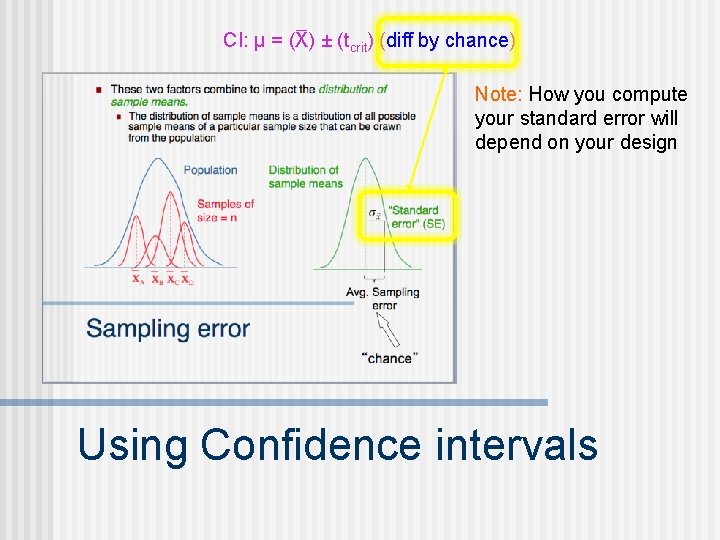
CI: μ = (X) ± (tcrit) (diff by chance) Note: How you compute your standard error will depend on your design Using Confidence intervals

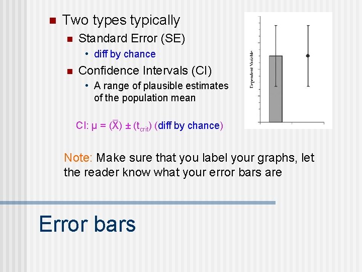
n Two types typically n Standard Error (SE) • diff by chance n Confidence Intervals (CI) • A range of plausible estimates of the population mean CI: μ = (X) ± (tcrit) (diff by chance) Note: Make sure that you label your graphs, let the reader know what your error bars are Error bars

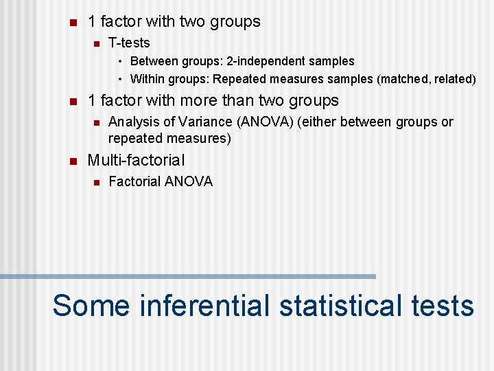
n 1 factor with two groups n T-tests • Between groups: 2 -independent samples • Within groups: Repeated measures samples (matched, related) n 1 factor with more than two groups n n Analysis of Variance (ANOVA) (either between groups or repeated measures) Multi-factorial n Factorial ANOVA Some inferential statistical tests

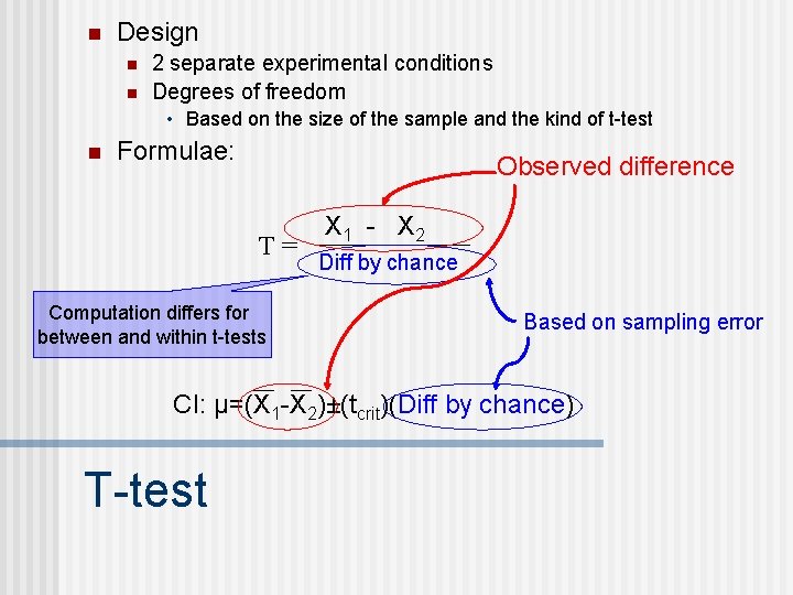
n Design n n 2 separate experimental conditions Degrees of freedom • Based on the size of the sample and the kind of t-test n Formulae: Observed difference T= Computation differs for between and within t-tests X 1 - X 2 Diff by chance Based on sampling error CI: μ=(X 1 -X 2)±(tcrit)(Diff by chance) T-test

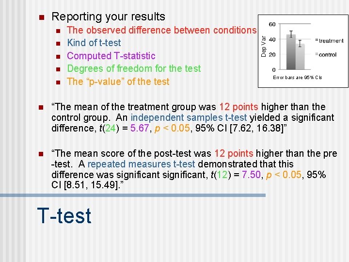
Reporting your results n n n The observed difference between conditions Kind of t-test Computed T-statistic Degrees of freedom for the test The “p-value” of the test Dep Var n Error bars are 95% CIs n “The mean of the treatment group was 12 points higher than the control group. An independent samples t-test yielded a significant difference, t(24) = 5. 67, p < 0. 05, 95% CI [7. 62, 16. 38]” n “The mean score of the post-test was 12 points higher than the pre -test. A repeated measures t-test demonstrated that this difference was significant, t(12) = 7. 50, p < 0. 05, 95% CI [8. 51, 15. 49]. ” T-test

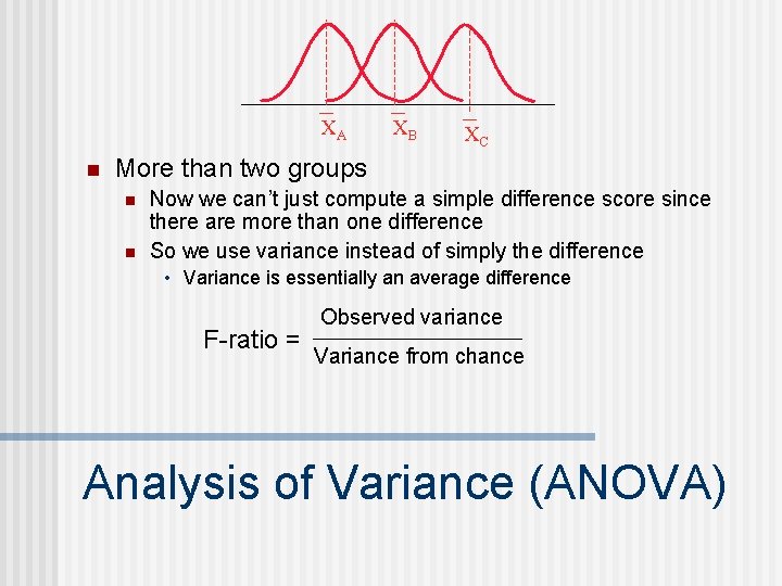
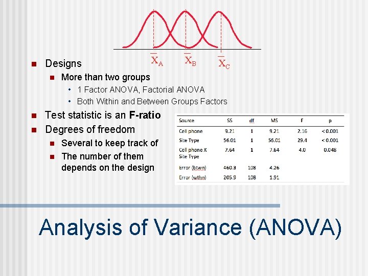
XA n XB XC More than two groups n n Now we can’t just compute a simple difference score since there are more than one difference So we use variance instead of simply the difference • Variance is essentially an average difference F-ratio = Observed variance Variance from chance Analysis of Variance (ANOVA)

n Designs n XA XB XC More than two groups • 1 Factor ANOVA, Factorial ANOVA • Both Within and Between Groups Factors n n Test statistic is an F-ratio Degrees of freedom n n Several to keep track of The number of them depends on the design Analysis of Variance (ANOVA)

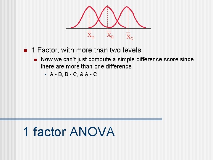
XA n XB XC 1 Factor, with more than two levels n Now we can’t just compute a simple difference score since there are more than one difference • A - B, B - C, & A - C 1 factor ANOVA

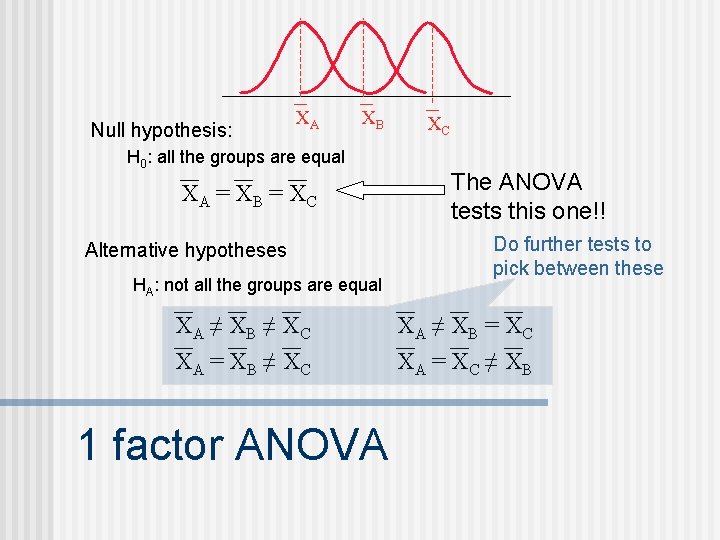
Null hypothesis: XA XB H 0: all the groups are equal XA = X B = X C Alternative hypotheses HA: not all the groups are equal XA ≠ X B ≠ X C XA = X B ≠ X C 1 factor ANOVA XC The ANOVA tests this one!! Do further tests to pick between these XA ≠ X B = X C XA = X C ≠ X B

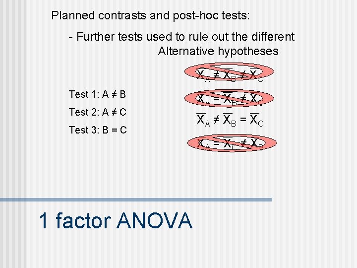
Planned contrasts and post-hoc tests: - Further tests used to rule out the different Alternative hypotheses XA ≠ X B ≠ X C Test 1: A ≠ B Test 2: A ≠ C Test 3: B = C XA = X B ≠ X C XA ≠ X B = X C XA = X C ≠ X B 1 factor ANOVA

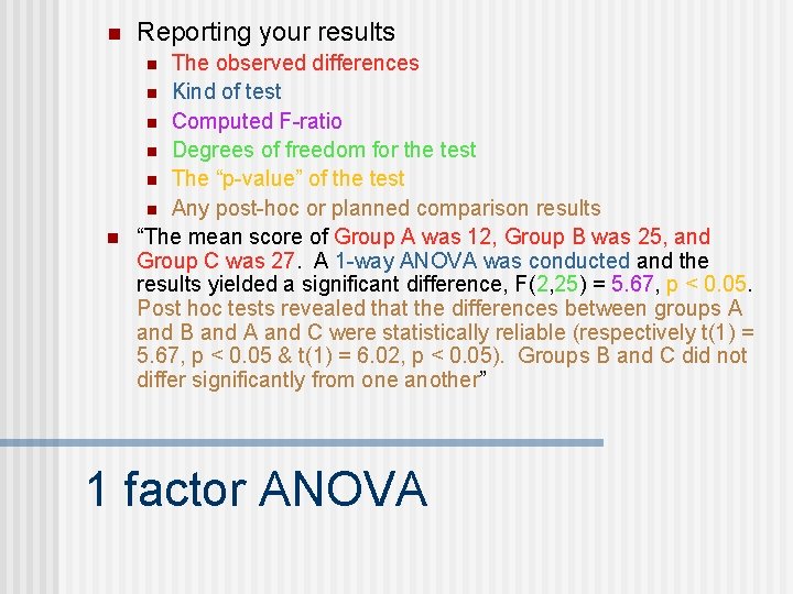
n Reporting your results The observed differences n Kind of test n Computed F-ratio n Degrees of freedom for the test n The “p-value” of the test n Any post-hoc or planned comparison results “The mean score of Group A was 12, Group B was 25, and Group C was 27. A 1 -way ANOVA was conducted and the results yielded a significant difference, F(2, 25) = 5. 67, p < 0. 05. Post hoc tests revealed that the differences between groups A and B and A and C were statistically reliable (respectively t(1) = 5. 67, p < 0. 05 & t(1) = 6. 02, p < 0. 05). Groups B and C did not differ significantly from one another” n n 1 factor ANOVA

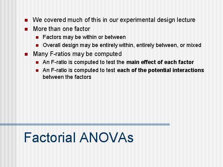
n n We covered much of this in our experimental design lecture More than one factor n n n Factors may be within or between Overall design may be entirely within, entirely between, or mixed Many F-ratios may be computed n n An F-ratio is computed to test the main effect of each factor An F-ratio is computed to test each of the potential interactions between the factors Factorial ANOVAs

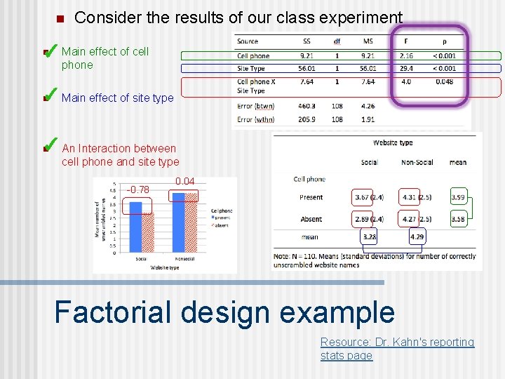
n Consider the results of our class experiment ✓ Main effect of cell n phone ✓ Main effect of site type n ✓ An Interaction between n cell phone and site type -0. 78 0. 04 Factorial design example Resource: Dr. Kahn's reporting stats page

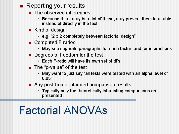
n Reporting your results n The observed differences • Because there may be a lot of these, may present them in a table instead of directly in the text n Kind of design • e. g. “ 2 x 2 completely between factorial design” n Computed F-ratios • May see separate paragraphs for each factor, and for interactions n Degrees of freedom for the test • Each F-ratio will have its own set of df’s n The “p-value” of the test • May want to just say “all tests were tested with an alpha level of 0. 05” n Any post-hoc or planned comparison results • Typically only theoretically interesting comparisons are presented Factorial ANOVAs