Statistical aspects of Higgs analyses W Verkerke NIKHEF

Statistical aspects of Higgs analyses W. Verkerke (NIKHEF)

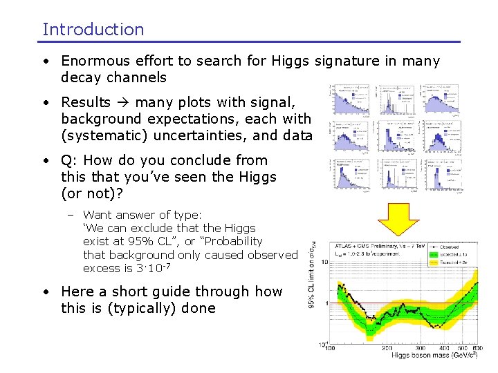
Introduction • Enormous effort to search for Higgs signature in many decay channels • Results many plots with signal, background expectations, each with (systematic) uncertainties, and data • Q: How do you conclude from this that you’ve seen the Higgs (or not)? – Want answer of type: ‘We can exclude that the Higgs exist at 95% CL”, or “Probability that background only caused observed excess is 3·10 -7 • Here a short guide through how this is (typically) done

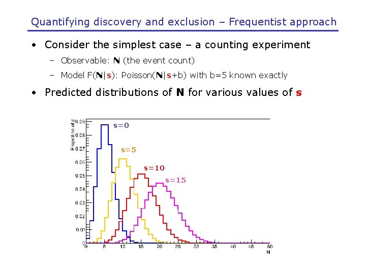
Quantifying discovery and exclusion – Frequentist approach • Consider the simplest case – a counting experiment – Observable: N (the event count) – Model F(N|s): Poisson(N|s+b) with b=5 known exactly • Predicted distributions of N for various values of s s=0 s=5 s=10 s=15

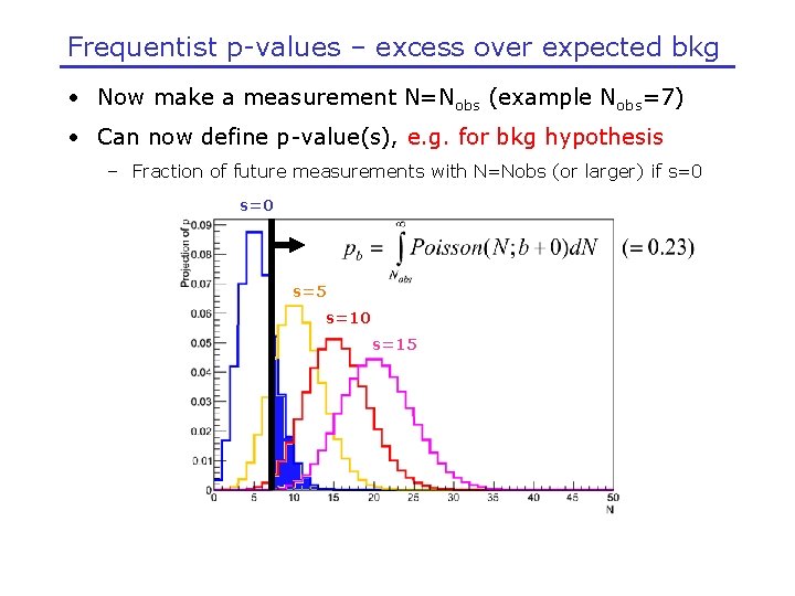
Frequentist p-values – excess over expected bkg • Now make a measurement N=Nobs (example Nobs=7) • Can now define p-value(s), e. g. for bkg hypothesis – Fraction of future measurements with N=Nobs (or larger) if s=0 s=5 s=10 s=15

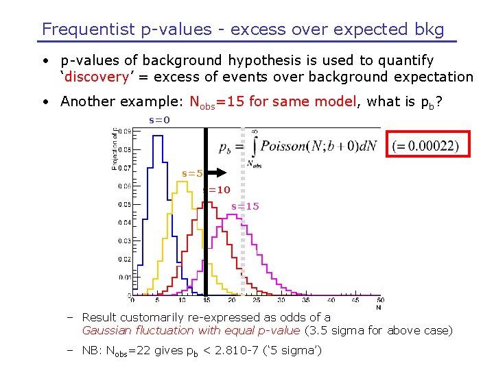
Frequentist p-values - excess over expected bkg • p-values of background hypothesis is used to quantify ‘discovery’ = excess of events over background expectation • Another example: Nobs=15 for same model, what is pb? s=0 s=5 s=10 s=15 – Result customarily re-expressed as odds of a Gaussian fluctuation with equal p-value (3. 5 sigma for above case) – NB: Nobs=22 gives pb < 2. 810 -7 (‘ 5 sigma’)

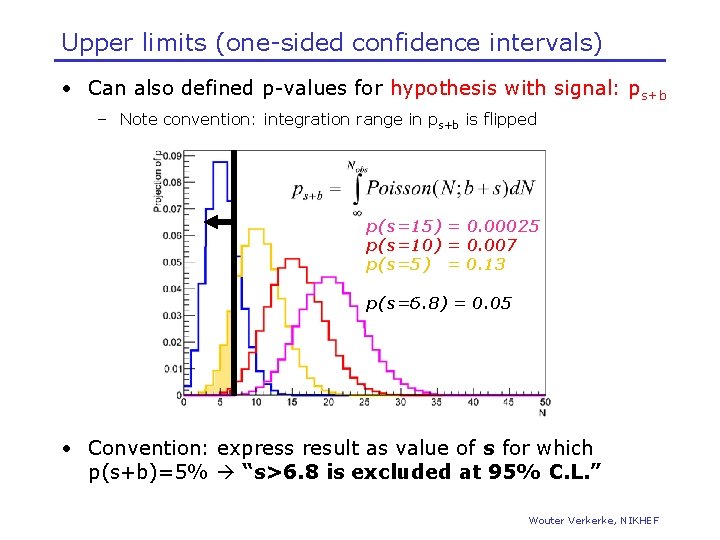
Upper limits (one-sided confidence intervals) • Can also defined p-values for hypothesis with signal: ps+b – Note convention: integration range in ps+b is flipped p(s=15) = 0. 00025 p(s=10) = 0. 007 p(s=5) = 0. 13 p(s=6. 8) = 0. 05 • Convention: express result as value of s for which p(s+b)=5% “s>6. 8 is excluded at 95% C. L. ” Wouter Verkerke, NIKHEF

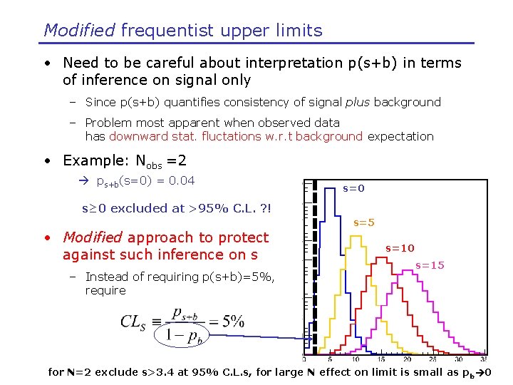
Modified frequentist upper limits • Need to be careful about interpretation p(s+b) in terms of inference on signal only – Since p(s+b) quantifies consistency of signal plus background – Problem most apparent when observed data has downward stat. fluctations w. r. t background expectation • Example: Nobs =2 ps+b(s=0) = 0. 04 s=0 s≥ 0 excluded at >95% C. L. ? ! • Modified approach to protect against such inference on s – Instead of requiring p(s+b)=5%, require s=5 s=10 s=15 for N=2 exclude s>3. 4 at 95% C. L. s, for large N effect on limit is small as p b 0

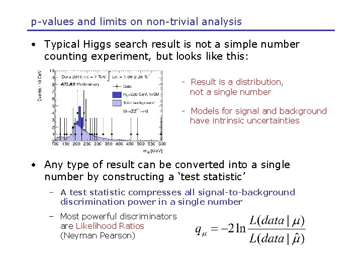
p-values and limits on non-trivial analysis • Typical Higgs search result is not a simple number counting experiment, but looks like this: - Result is a distribution, not a single number - Models for signal and background have intrinsic uncertainties • Any type of result can be converted into a single number by constructing a ‘test statistic’ – A test statistic compresses all signal-to-background discrimination power in a single number – Most powerful discriminators are Likelihood Ratios (Neyman Pearson)

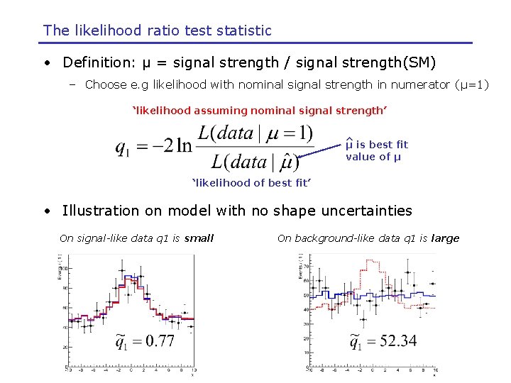
The likelihood ratio test statistic • Definition: μ = signal strength / signal strength(SM) – Choose e. g likelihood with nominal signal strength in numerator (μ=1) ‘likelihood assuming nominal signal strength’ ^ is best fit μ value of μ ‘likelihood of best fit’ • Illustration on model with no shape uncertainties On signal-like data q 1 is small On background-like data q 1 is large

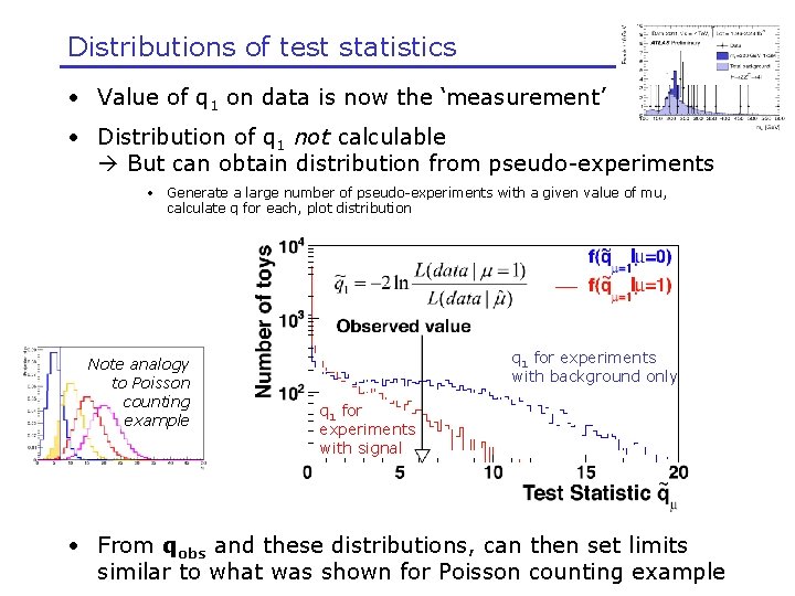
Distributions of test statistics • Value of q 1 on data is now the ‘measurement’ • Distribution of q 1 not calculable But can obtain distribution from pseudo-experiments • Generate a large number of pseudo-experiments with a given value of mu, calculate q for each, plot distribution Note analogy to Poisson counting example q 1 for experiments with background only q 1 for experiments with signal • From qobs and these distributions, can then set limits similar to what was shown for Poisson counting example

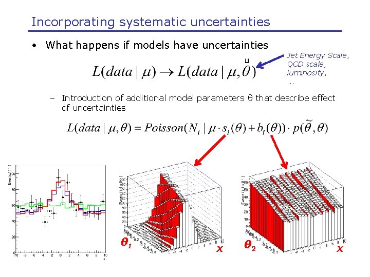
Incorporating systematic uncertainties • What happens if models have uncertainties Jet Energy Scale, QCD scale, luminosity, . . . – Introduction of additional model parameters θ that describe effect of uncertainties θ 1 x θ 2 x

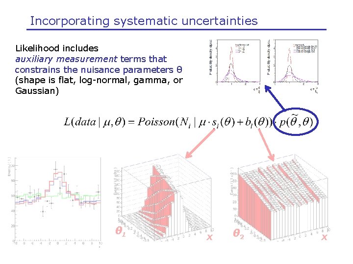
Incorporating systematic uncertainties Likelihood includes auxiliary measurement terms that constrains the nuisance parameters θ (shape is flat, log-normal, gamma, or Gaussian) θ 1 x θ 2 x

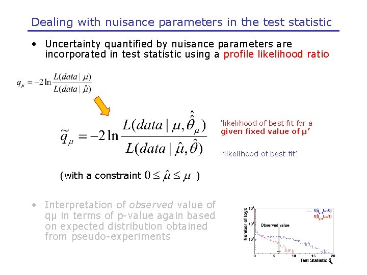
Dealing with nuisance parameters in the test statistic • Uncertainty quantified by nuisance parameters are incorporated in test statistic using a profile likelihood ratio ‘likelihood of best fit for a given fixed value of μ’ ‘likelihood of best fit’ (with a constraint ) • Interpretation of observed value of qμ in terms of p-value again based on expected distribution obtained from pseudo-experiments

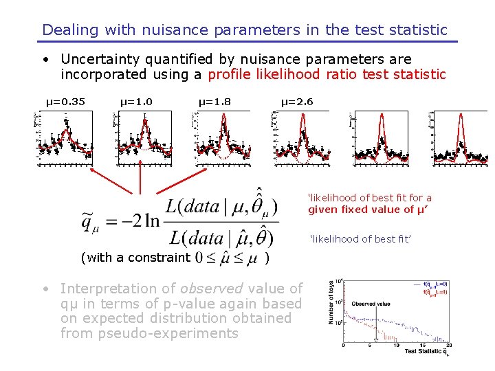
Dealing with nuisance parameters in the test statistic • Uncertainty quantified by nuisance parameters are incorporated using a profile likelihood ratio test statistic μ=0. 35 μ=1. 0 μ=1. 8 μ=2. 6 ‘likelihood of best fit for a given fixed value of μ’ ‘likelihood of best fit’ (with a constraint ) • Interpretation of observed value of qμ in terms of p-value again based on expected distribution obtained from pseudo-experiments

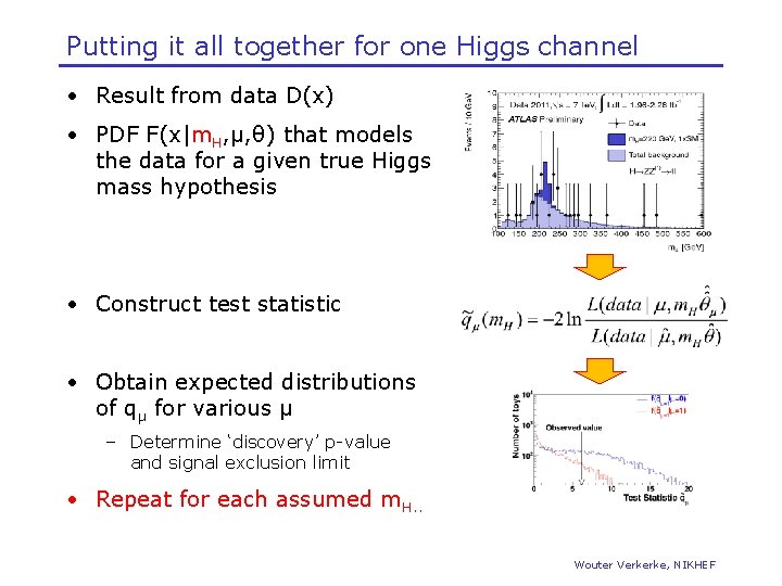
Putting it all together for one Higgs channel • Result from data D(x) • PDF F(x|m. H, μ, θ) that models the data for a given true Higgs mass hypothesis • Construct test statistic • Obtain expected distributions of qμ for various μ – Determine ‘discovery’ p-value and signal exclusion limit • Repeat for each assumed m. H. . Wouter Verkerke, NIKHEF

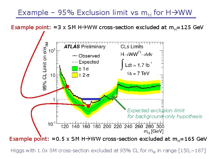
Example – 95% Exclusion limit vs m. H for H WW Example point: ≈3 x SM H WW cross-section excluded at m. H=125 Ge. V Expected exclusion limit for background-only hypothesis Example point: ≈0. 5 x SM H WW cross-section excluded at m. H=165 Ge. V Higgs with 1. 0 x SM cross-section excluded at 95% CL for m H in range [150, ~187]

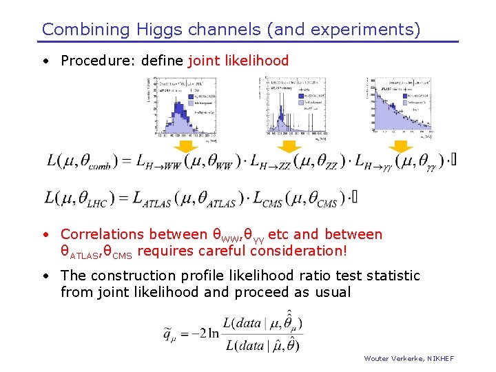
Combining Higgs channels (and experiments) • Procedure: define joint likelihood • Correlations between θWW, θγγ etc and between θATLAS, θCMS requires careful consideration! • The construction profile likelihood ratio test statistic from joint likelihood and proceed as usual Wouter Verkerke, NIKHEF

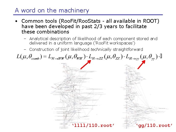
A word on the machinery • Common tools (Roo. Fit/Roo. Stats - all available in ROOT) have been developed in past 2/3 years to facilitate these combinations – Analytical description of likelihood of each component stored and delivered in a uniform language (‘Roo. Fit workspaces’) – Construction of joint likelihood technically straightforward ‘llll/110. root’ ‘gg/110. root’ Wouter Verkerke, NIKHEF

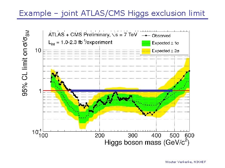
Example – joint ATLAS/CMS Higgs exclusion limit Wouter Verkerke, NIKHEF

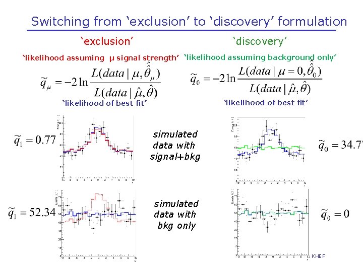
Switching from ‘exclusion’ to ‘discovery’ formulation ‘exclusion’ ‘discovery’ ‘likelihood assuming μ signal strength’ ‘likelihood assuming background only’ ‘likelihood of best fit’ simulated data with signal+bkg simulated data with bkg only Wouter Verkerke, NIKHEF

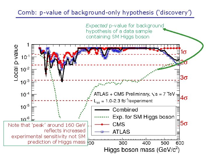
Comb: p-value of background-only hypothesis (‘discovery’) Expected p-value for background hypothesis of a data sample containing SM Higgs boson Note that ‘peak’ around 160 Ge. V reflects increased experimental sensitivity not SM prediction of Higgs mass

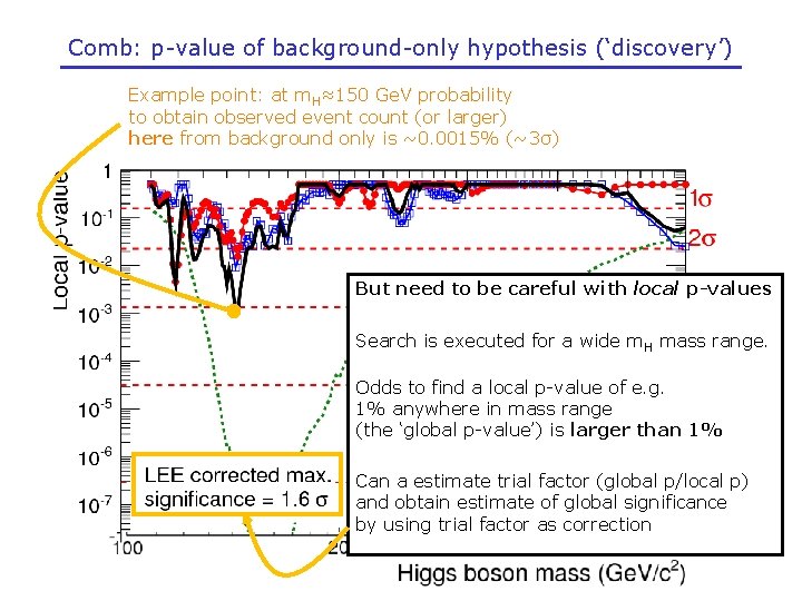
Comb: p-value of background-only hypothesis (‘discovery’) Example point: at m. H≈150 Ge. V probability to obtain observed event count (or larger) here from background only is ~0. 0015% (~3σ) But need to be careful with local p-values Search is executed for a wide m. H mass range. Odds to find a local p-value of e. g. 1% anywhere in mass range (the ‘global p-value’) is larger than 1% Can a estimate trial factor (global p/local p) and obtain estimate of global significance by using trial factor as correction

Conclusions • We are early awaiting more data! Wouter Verkerke, NIKHEF