Statistical analyses SPSS Statistical analysis program It is

Statistical analyses

SPSS Statistical analysis program It is an analytical software recognized by the scientific world (e. g. : the Microsoft Excel program is not recognized by the scientific world)

SPSS Let’s start the SPSS software! Paste the data onto the DATA VIEW window! It has two windows, one of them contains the data (DATA VIEW), and the types of the variables must be given in the other one (VARIABLES). Exact coding of variables is the basis of successful SPSS use.

Basics of computer-based analysis

Types of data Measurable data Differences between data are equal E. g. interval scale How old are you? How much is your weight? Ordinal data Data originating from gradation Special type: reletad gradation positions Nominal scale The data are replaced by numbers. E. g. Gender? 1. Male 2. Female The data do not signal order The data cannot be added

Statistical procedures Descriptive statistics If we analyze actual persons, that is population = samples Statistical indicators Frequencies Central tendency Dispersion Correlation

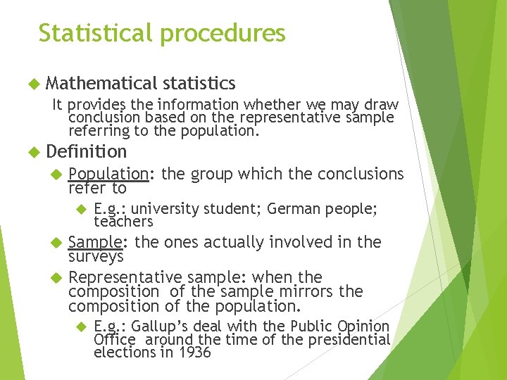
Statistical procedures Mathematical statistics It provides the information whether we may draw conclusion based on the representative sample referring to the population. Definition Population: the group which the conclusions refer to E. g. : university student; German people; teachers Sample: the ones actually involved in the surveys Representative sample: when the composition of the sample mirrors the composition of the population. E. g. : Gallup’s deal with the Public Opinion Office around the time of the presidential elections in 1936

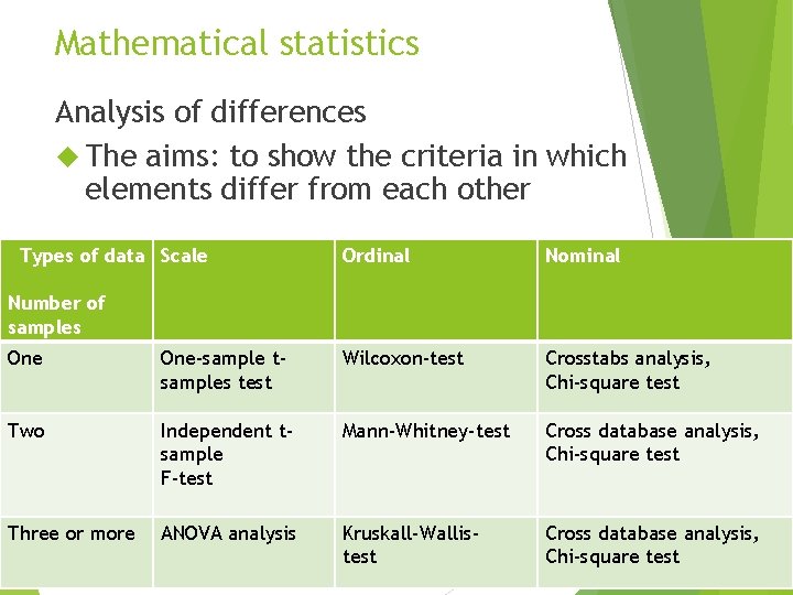
Mathematical statistics Analysis of differences The aims: to show the criteria in which elements differ from each other Types of data Scale Ordinal Nominal Number of samples One-sample tsamples test Wilcoxon-test Crosstabs analysis, Chi-square test Two Independent tsample F-test Mann-Whitney-test Cross database analysis, Chi-square test Three or more ANOVA analysis Kruskall-Wallistest Cross database analysis, Chi-square test

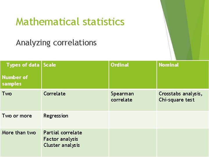
Mathematical statistics Analyzing correlations Types of data Scale Ordinal Nominal Spearman correlate Crosstabs analysis, Chi-square test Number of samples Two Correlate Two or more Regression More than two Partial correlate Factor analysis Cluster analysis

Descriptive statistics

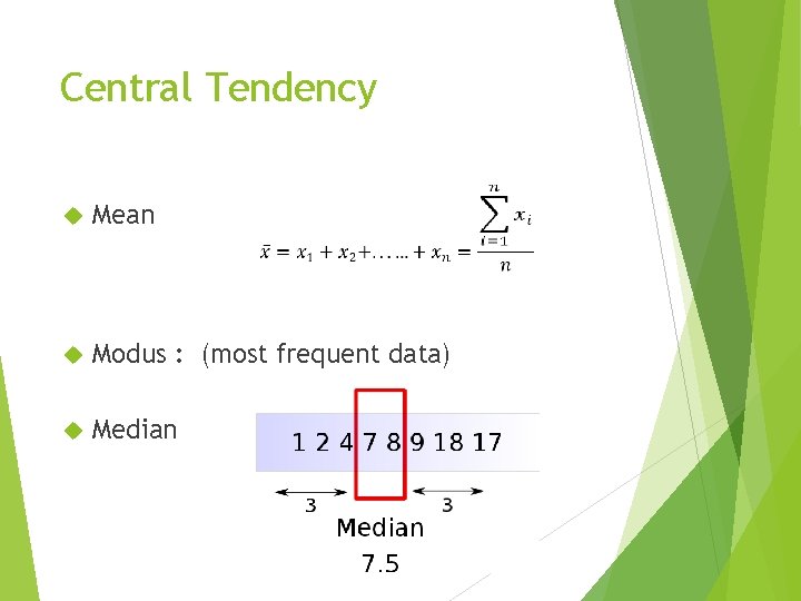
Central Tendency Mean Modus : (most frequent data) Median

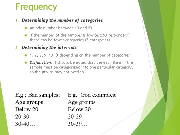
Frequency 1. 2. Determining the number of categories An odd number between 10 and 20 If the number of the samples is low (e. g. 50 responders) there can be fewer categories (7 categories) Determining the intervals 1, 2, 3, 5, 10 depending on the number of categories Disjunction: It should be noted that the each item in the sample must be categorized into one particular category, so the groups may not overlap. E. g. : Bad samples: Age groups Below 20 20 -30 30 -40… E. g. : God examples: Age groups Below 20 20 -29 30 -39…

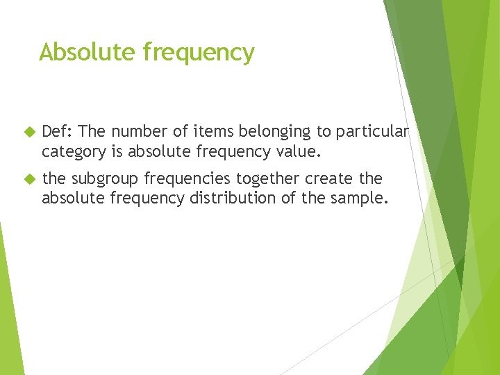
Absolute frequency Def: The number of items belonging to particular category is absolute frequency value. the subgroup frequencies together create the absolute frequency distribution of the sample.

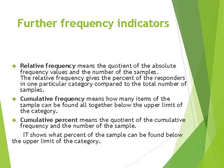
Further frequency indicators Relative frequency means the quotient of the absolute frequency values and the number of the samples. The relative frequency gives the percent of the responders in one particular category compared to the total number of samples. Cumulative frequency means how many items of the sample can be found all together below the upper limit of the category. Cumulative percent means the quotient of the cumulative frequency and the number of the sample. IT shows what percent of the sample can be found below the upper limit of the category.

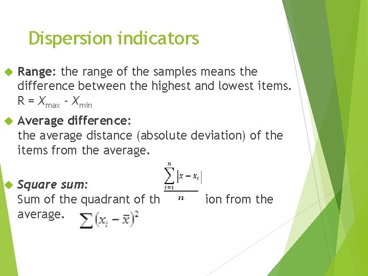
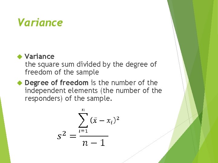
Dispersion indicators Range: the range of the samples means the difference between the highest and lowest items. R = Xmax - Xmin Average difference: the average distance (absolute deviation) of the items from the average. Square sum: Sum of the quadrant of the deviation from the average.

Variance the square sum divided by the degree of freedom of the sample Degree of freedom is the number of the independent elements (the number of the responders) of the sample.

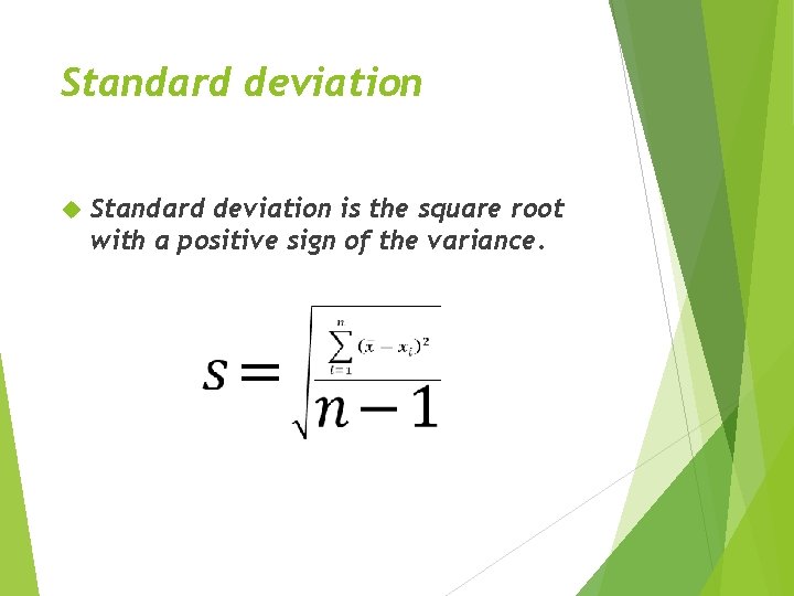
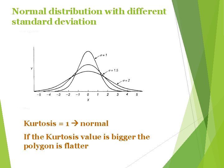
Standard deviation is the square root with a positive sign of the variance.

Theorem More than 2/3 of the data belong to a 1 standard deviation extending to the positive and negative directions from the mean. More than 90% of the data belong to a 2 standard deviation taken from the mean. More than 90% of the data belong to a 3 standard deviation taken from the mean.

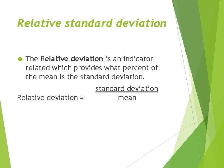
Relative standard deviation The Relative deviation is an indicator related which provides what percent of the mean is the standard deviation. Relative deviation = standard deviation mean

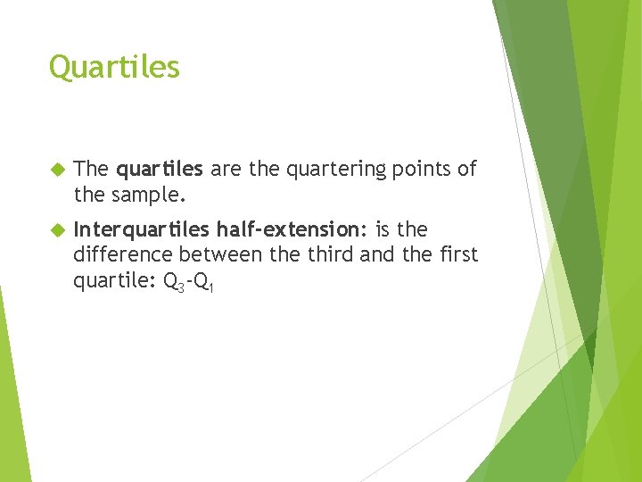
Quartiles The quartiles are the quartering points of the sample. Interquartiles half-extension: is the difference between the third and the first quartile: Q 3 -Q 1

Interrelations

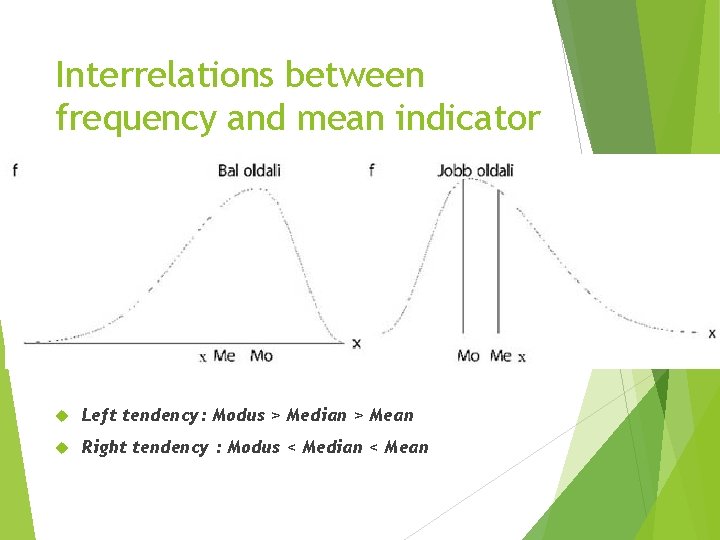
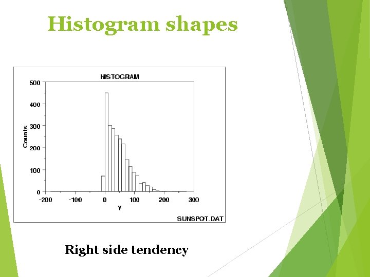
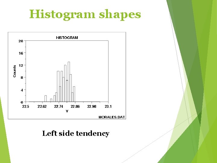
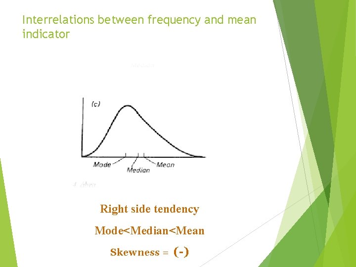
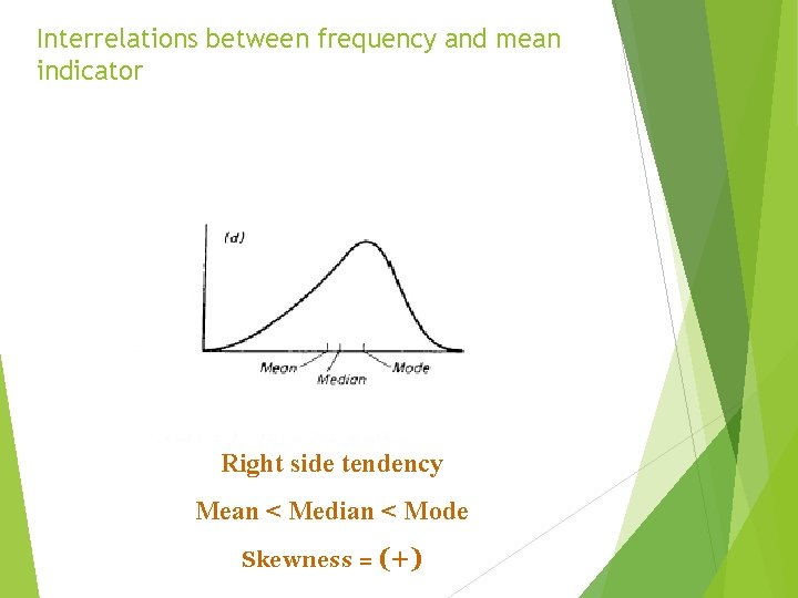
Interrelations between frequency and mean indicator Left tendency: Modus > Median > Mean Right tendency : Modus < Median < Mean

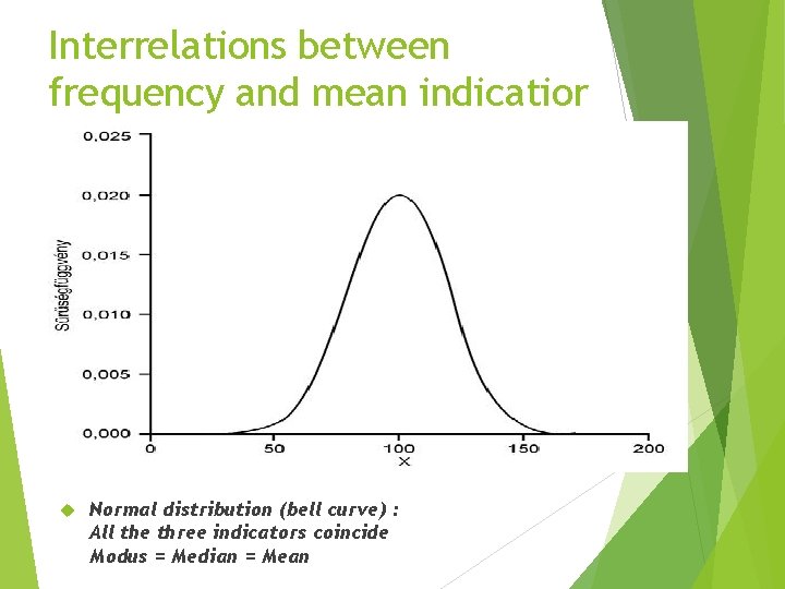
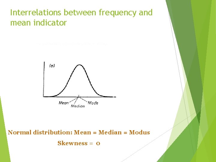
Interrelations between frequency and mean indicatior Normal distribution (bell curve) : All the three indicators coincide Modus = Median = Mean

Mathematical statistics

Relations examinations

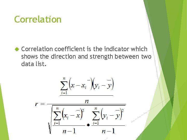
Correlation coefficient is the indicator which shows the direction and strength between two data list.

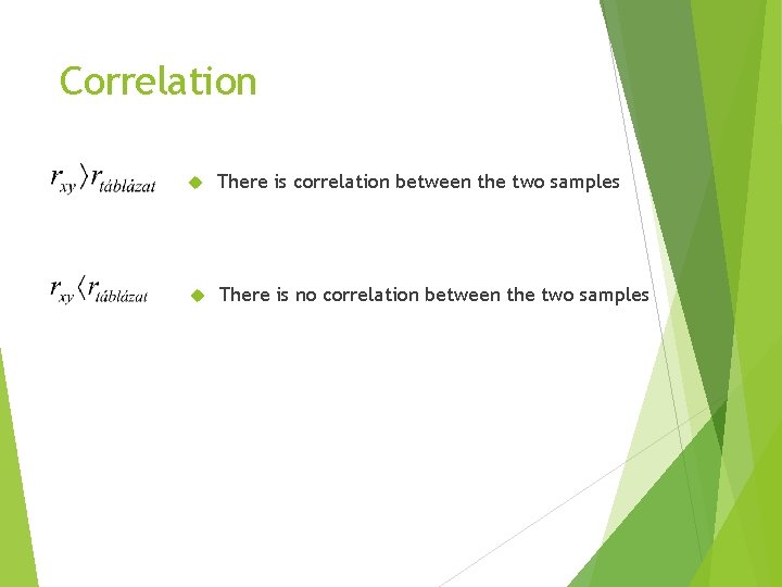
Correlation There is correlation between the two samples There is no correlation between the two samples

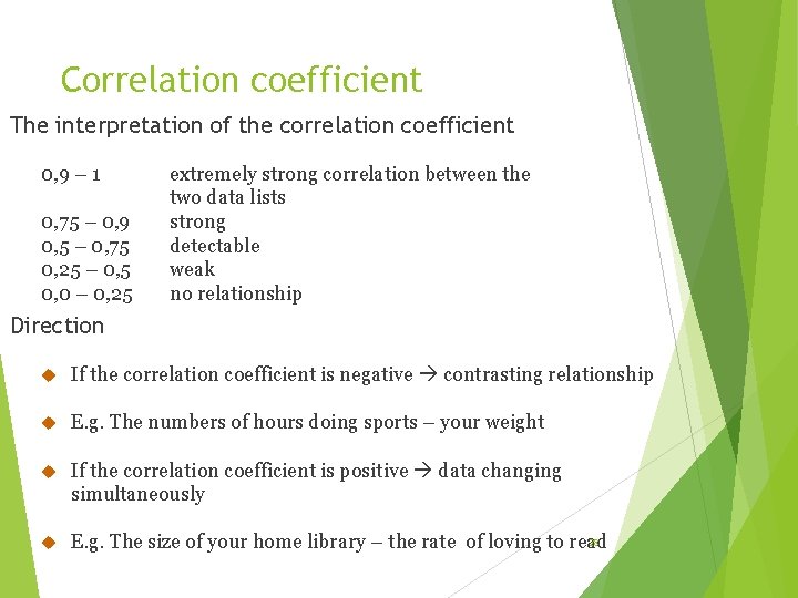
Correlation coefficient The interpretation of the correlation coefficient 0, 9 – 1 0, 75 – 0, 9 0, 5 – 0, 75 0, 25 – 0, 5 0, 0 – 0, 25 extremely strong correlation between the two data lists strong detectable weak no relationship Direction If the correlation coefficient is negative contrasting relationship E. g. The numbers of hours doing sports – your weight If the correlation coefficient is positive data changing simultaneously 28 E. g. The size of your home library – the rate of loving to read

Relationship between/among variables – Crosstabs – illustrating the distribution of two nominal or ordinal variables on the same chart.

Crosstabs- Chi-square It is an indicator which shows whether the correlations in the cross tabs are valid only for the samples or for the population as well. It cannot be used efficiently if the value is less then 5 in more than 20% of the cells.

Hypothesis analyses It is a method to decide whether the differences in data are significant or random.

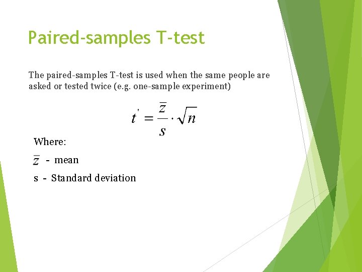
Paired-samples T-test The paired-samples T-test is used when the same people are asked or tested twice (e. g. one-sample experiment) Where: - mean s - Standard deviation

Paired-samples T-test Match the t-number with the value of the „Critical values of the t-distribution” chart If t’ > t chart the different is significant If t’ < t chart the different is random

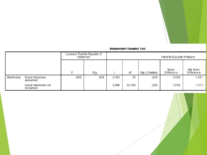
T-test with computer It is not necessary use the „Critical values of the t-distribution” chart, because most software provides the „p” value (Signif of t, Sig. Level). The „p” shows what percent is the failure rate. If „p”<0. 05 (5%) then the difference is significant

Independent t-test H 0: two independent samples taken from the same population. (H 0 definition: the zero hypothesis is that the difference is random ) This type of test can only can be conductived if the variances of the two groups not too different. The F-test can give the answer.

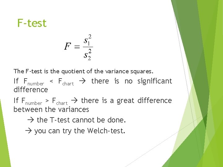
F-test The F-test is the quotient of the variance squares. If Fnumber < Fchart there is no significant difference If Fnumber > Fchart there is a great difference between the variances the T-test cannot be done. you can try the Welch-test.

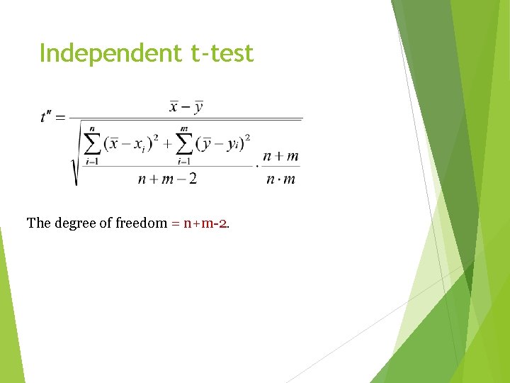
Independent t-test The degree of freedom = n+m-2.

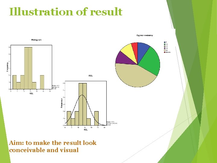
Illustration of result Aim: to make the result look conceivable and visual

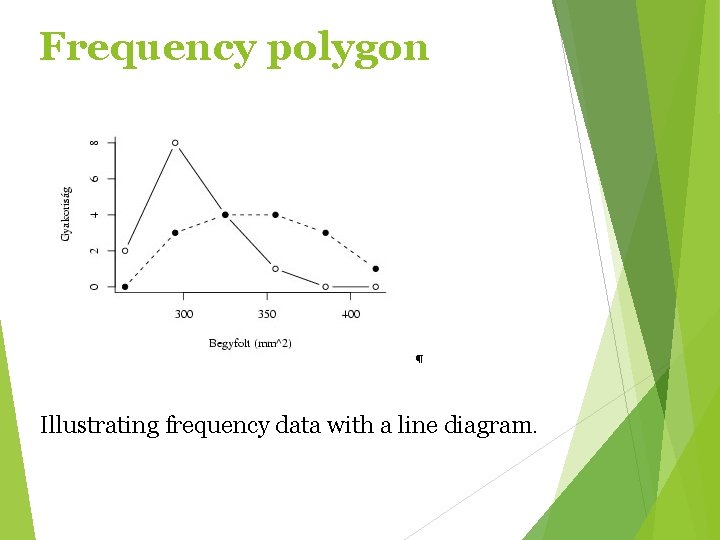
Frequency polygon Illustrating frequency data with a line diagram.

Histogram Illustrating frequency data with a bar diagram. The title of the X axis is intervals.

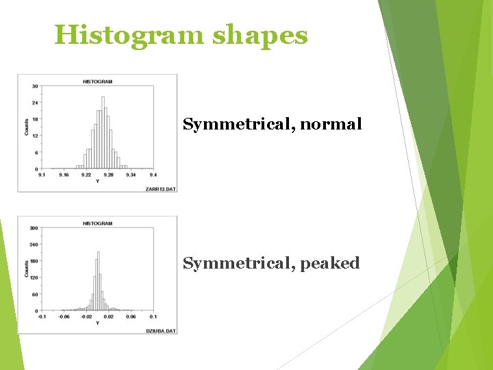
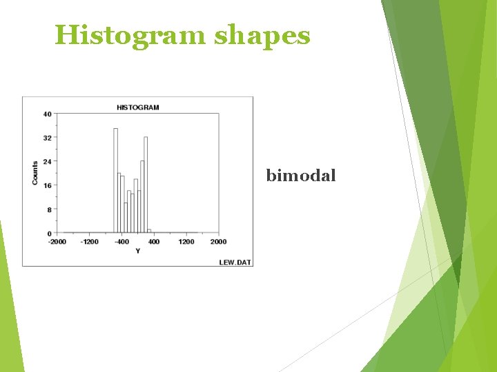
Histogram shapes Symmetrical, normal Symmetrical, peaked

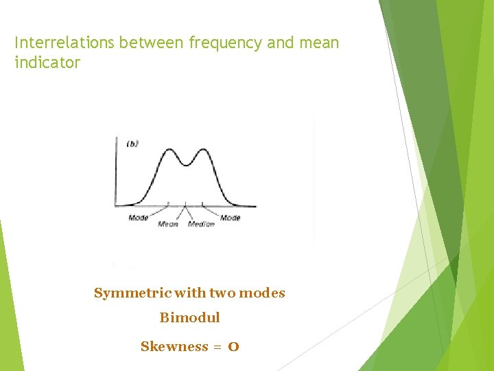
Histogram shapes bimodal

Histogram shapes Right side tendency

Histogram shapes Left side tendency

Interrelations between frequency and mean indicator Normal distribution: Mean = Median = Modus Skewness = 0

Interrelations between frequency and mean indicator Symmetric with two modes Bimodul Skewness = 0

Interrelations between frequency and mean indicator Right side tendency Mode<Median<Mean Skewness = (-)

Interrelations between frequency and mean indicator Right side tendency Mean < Median < Mode Skewness = (+)

Normal distribution with different standard deviation Kurtosis = 1 normal If the Kurtosis value is bigger the polygon is flatter