SQL Naveen Ashish Calit 2 ICS UC Irvine

SQL Naveen Ashish Calit 2 & ICS UC Irvine

SQL -- historical Perspective l Dr. Edgar Codd (IBM) l l l “A Relational Model of Data for Large Shared Data Banks" CACM June 1970 Standardized 1986 by ANSI --- SQL 1 l Revised in 1992 ---SQL 2. l Approx 580 page document describing syntax and semantics l 1999: SQL 3 l 2003: 2003 SQL 3 l l Players l l l IBM, Relational Software (Oracle), …. Every vendor has a slightly different version of SQL Simple and declarative

Portability l l l Many different implementations Need not completely conform to standard Own specialized versions l l PL/SQL, SQL PL, Transact-SQL, …. . Portability (of application) in one SQL implementation to another is usually messy l l Standard implementation left to vendor Not break backward compatibility for user base l “Vendor Lock-in”

SQL in Different Roles l l l Data Definition language: l allows users to describe the relations and constraints. Constraint specification language: l commands to specify constraints ensured by DBMS Query language: l relationally complete, supports aggregation and grouping l declarative -- you specify what you want and not how to retrieve, easy to learn and program Updates in SQL: l allows users to insert, delete and modify tables View definition language: l commands to define rules l updates through views generally not supported

SQL in Different Roles l Embedded SQL: l l l has been embedded in a variety of host languages--C, C++, PERL, Smalltalk, Java (vendor dependent) Impedance mismatch: SQL manipulates relations that are sets--- programming languages do not handle sets as efficiently. Transaction Control: l commands to specify beginning and end of transactions.

SQL as Data Definition Language l Allows users to l specify the relation schemas l domain of each attribute l integrity constraints l set of indices to be maintained on the relation l we will learn what indices are later l security and authorization information for each relation l the physical storage structure for each relation on disk.

Domain Types l l l char(n): fixed length char string varchar(n): variable length char string int or integer smallint numeric(p, d): fixed-point number of given precision real, double precision float(n): floats with a given precision date: containing year, month, date time: in hours, minutes and seconds Null value is part of each domain Define new domains: l create domain person-name char(20)

Schema Definition Create table r ( A 1 D 1 [not null] [default V 1] A 2 D 2 [not null] [default V 2] … An Dn [not null] [default Vn] <integrity constraint 1> <integrity constraint 2> … <integrity constraint k> ) Integrity constraints 1 … k could be: l l primary key candidate key foreign key check(predicate) specifies predicate that must be satisfied by each tuple

SQL as DDL create table Employee ( name char[15] age smallint sex (M, F) ss# integer spouse_ss# integer dept# integer ) l l not null Default value is Male default M not null Don’t allow null values Primary Key (ssno) Unique(spouse_ss#) • if dept# updated/deleted in Dept Check (age >=20 and age <=70) table, cascade update/delete to Foreign key (dept#) references Dept(dept#) Employee on delete cascade on update cascade • if null/default instead of cascade, null/default value taken by dangling tuples in Employee

SQL as DDL l l l l Attributes in primary key required to be not null Attributes in candidate key can take null values unless specified otherwise Unique constraint violated if two tuples have exactly same values for attributes in unique clause provided values are not null Null also permitted for attributes in foreign key. Foreign key constraint automatically satisfied if even one attribute in foreign key is null. Predicate in check clause can be very complex and can include SQL queries inside them Other DDL Statements: l l l drop table r alter table r add A D alter table r drop A

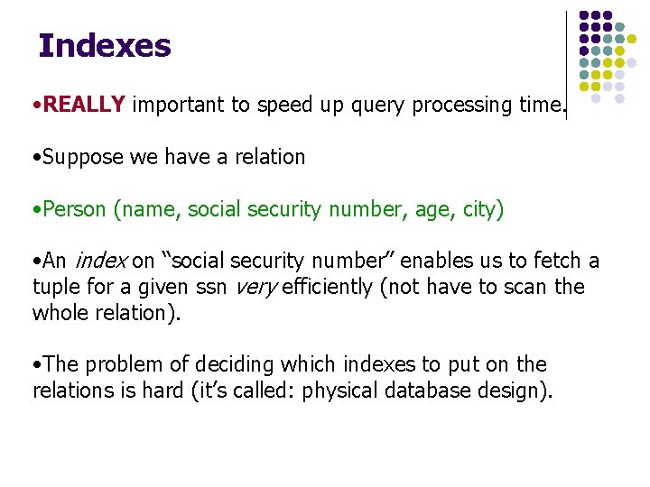
Indexes • REALLY important to speed up query processing time. • Suppose we have a relation • Person (name, social security number, age, city) • An index on “social security number” enables us to fetch a tuple for a given ssn very efficiently (not have to scan the whole relation). • The problem of deciding which indexes to put on the relations is hard (it’s called: physical database design).

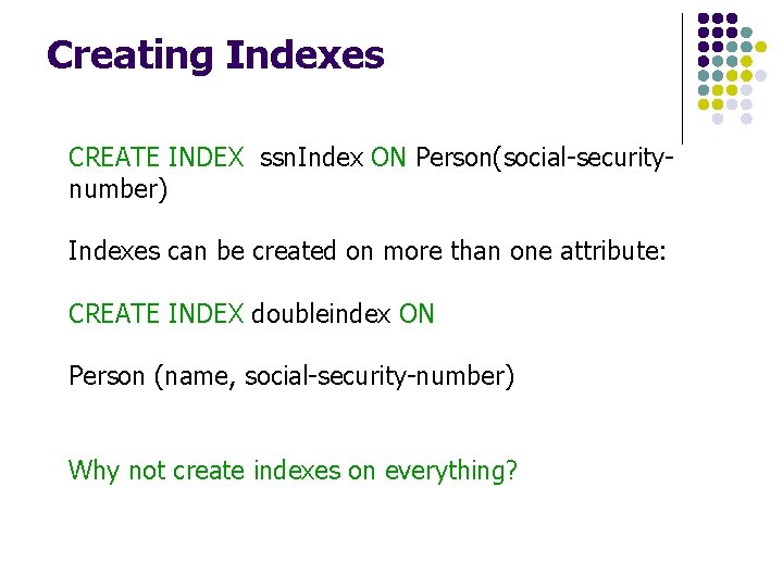
Creating Indexes CREATE INDEX ssn. Index ON Person(social-securitynumber) Indexes can be created on more than one attribute: CREATE INDEX doubleindex ON Person (name, social-security-number) Why not create indexes on everything?

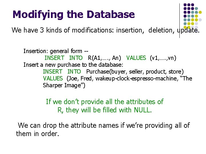
Modifying the Database We have 3 kinds of modifications: insertion, deletion, update. Insertion: general form -INSERT INTO R(A 1, …. , An) VALUES (v 1, …. , vn) Insert a new purchase to the database: INSERT INTO Purchase(buyer, seller, product, store) VALUES (Joe, Fred, wakeup-clock-espresso-machine, “The Sharper Image”) If we don’t provide all the attributes of R, they will be filled with NULL. We can drop the attribute names if we’re providing all of them in order.

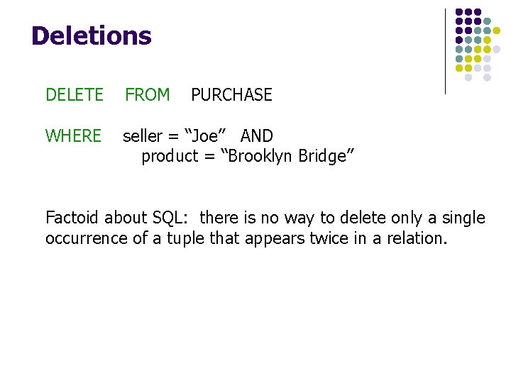
Deletions DELETE FROM PURCHASE WHERE seller = “Joe” AND product = “Brooklyn Bridge” Factoid about SQL: there is no way to delete only a single occurrence of a tuple that appears twice in a relation.

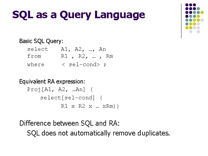
SQL as a Query Language Basic SQL Query: select A 1, A 2, …, An from R 1 , R 2, … , Rm where < sel-cond> ; Equivalent RA expression: Proj[A 1, A 2, …An] ( select[sel-cond] ( R 1 x R 2 x … x. Rm)) Difference between SQL and RA: SQL does not automatically remove duplicates.

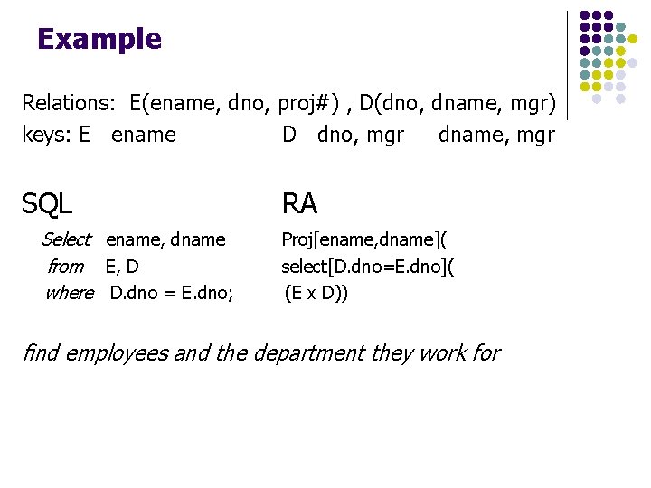
Example Relations: E(ename, dno, proj#) , D(dno, dname, mgr) keys: E ename D dno, mgr dname, mgr SQL Select ename, dname from E, D where D. dno = E. dno; RA Proj[ename, dname]( select[D. dno=E. dno]( (E x D)) find employees and the department they work for

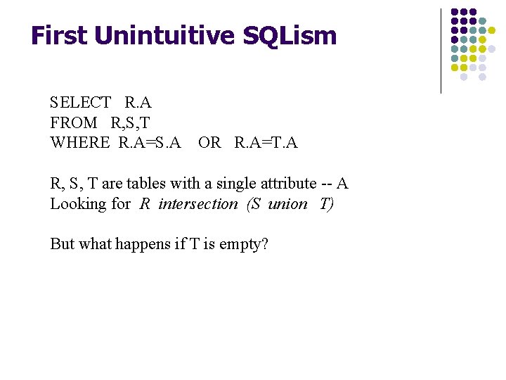
First Unintuitive SQLism SELECT R. A FROM R, S, T WHERE R. A=S. A OR R. A=T. A R, S, T are tables with a single attribute -- A Looking for R intersection (S union T) But what happens if T is empty?

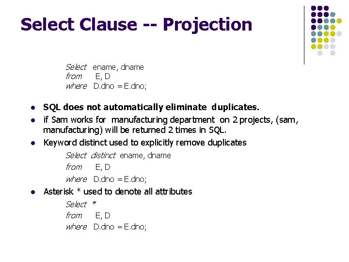
Select Clause -- Projection Select ename, dname from E, D where D. dno = E. dno; l l l SQL does not automatically eliminate duplicates. if Sam works for manufacturing department on 2 projects, (sam, manufacturing) will be returned 2 times in SQL. Keyword distinct used to explicitly remove duplicates Select distinct ename, dname from E, D where D. dno = E. dno; l Asterisk * used to denote all attributes Select * from E, D where D. dno = E. dno;

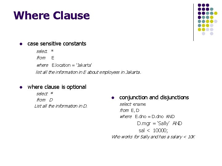
Where Clause l case sensitive constants select * from E where E. location = ‘Jakarta’ list all the information in E about employees in Jakarta. l where clause is optional select * from D List all the information in D. l conjunction and disjunctions select ename from E, D where E. dno = D. dno AND D. mgr = ‘Sally’ AND sal < 10000; Who works for Sally and has a salary < 10 K

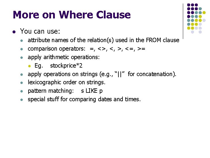
More on Where Clause l You can use: l l l l attribute names of the relation(s) used in the FROM clause comparison operators: =, <>, <, >, <=, >= apply arithmetic operations: l Eg. stockprice*2 apply operations on strings (e. g. , “||” for concatenation). lexicographic order on strings. pattern matching: s LIKE p special stuff for comparing dates and times.

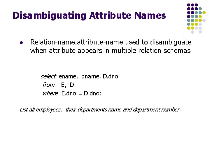
Disambiguating Attribute Names l Relation-name. attribute-name used to disambiguate when attribute appears in multiple relation schemas select ename, dname, D. dno from E, D where E. dno = D. dno; List all employees, their departments name and department number.

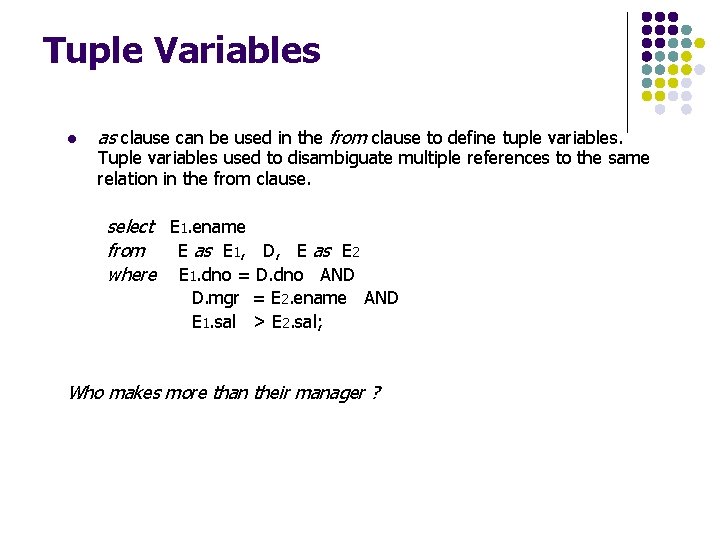
Tuple Variables l as clause can be used in the from clause to define tuple variables. Tuple variables used to disambiguate multiple references to the same relation in the from clause. select E 1. ename from E as E 1, D, E as E 2 where E 1. dno = D. dno AND D. mgr = E 2. ename AND E 1. sal > E 2. sal; Who makes more than their manager ?

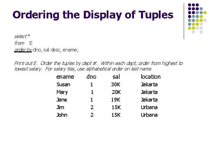
Ordering the Display of Tuples select * from E order by dno, sal desc, ename; Print out E. Order the tuples by dept #. Within each dept, order from highest to lowest salary. For salary ties, use alphabetical order on last name ename Susan Mary Jane Jim John dno sal 1 1 1 2 2 30 K 20 K 19 K 15 K location Jakarta Urbana

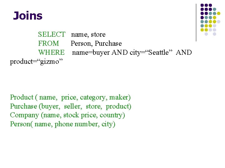
Joins SELECT name, store FROM Person, Purchase WHERE name=buyer AND city=“Seattle” AND product=“gizmo” Product ( name, price, category, maker) Purchase (buyer, seller, store, product) Company (name, stock price, country) Person( name, phone number, city)

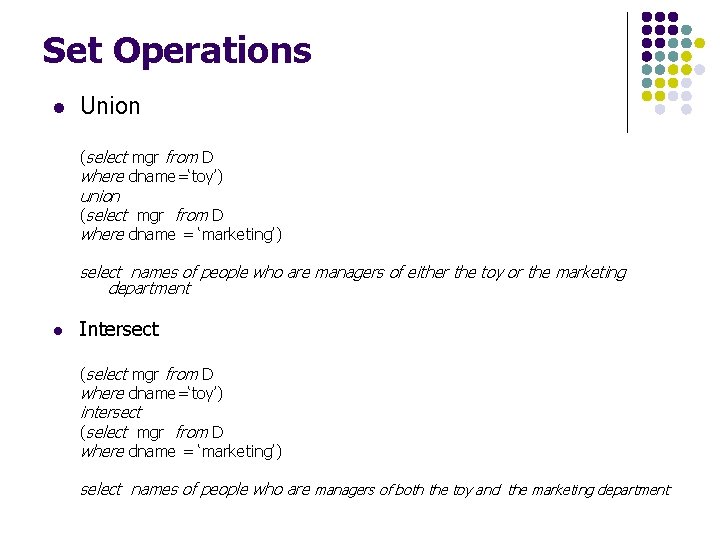
Set Operations l Union (select mgr from D where dname=‘toy’) union (select mgr from D where dname = ‘marketing’) select names of people who are managers of either the toy or the marketing department l Intersect (select mgr from D where dname=‘toy’) intersect (select mgr from D where dname = ‘marketing’) select names of people who are managers of both the toy and the marketing department

Set Operations l Except (select mgr from D where dname=‘toy’) except (select mgr from D where dname = ‘marketing’) l select names of people who are managers of toy department but not of marketing department

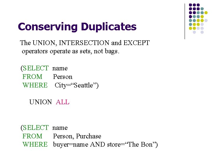
Conserving Duplicates The UNION, INTERSECTION and EXCEPT operators operate as sets, not bags. (SELECT name FROM Person WHERE City=“Seattle”) UNION ALL (SELECT name FROM Person, Purchase WHERE buyer=name AND store=“The Bon”)

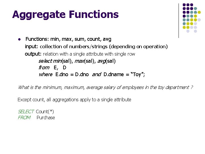
Aggregate Functions l Functions: min, max, sum, count, avg input: collection of numbers/strings (depending on operation) output: relation with a single attribute with single row select min(sal), max(sal), avg(sal) from E, D where E. dno = D. dno and D. dname = “Toy”; What is the minimum, maximum, average salary of employees in the toy department ? Except count, all aggregations apply to a single attribute SELECT Count(*) FROM Purchase

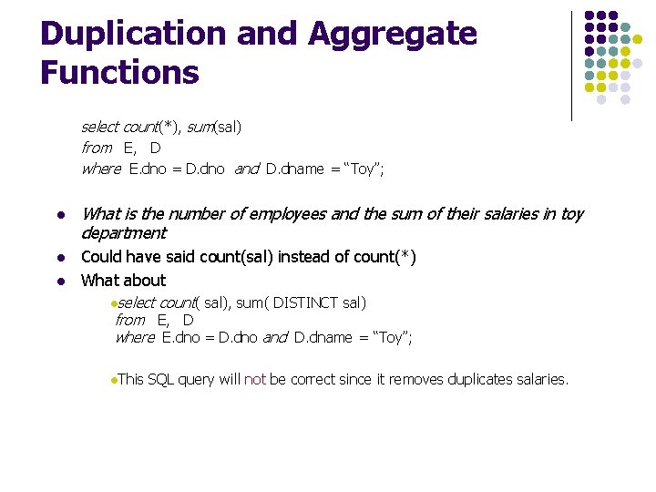
Duplication and Aggregate Functions select count(*), sum(sal) from E, D where E. dno = D. dno and D. dname = “Toy”; l l l What is the number of employees and the sum of their salaries in toy department Could have said count(sal) instead of count(*) What about lselect count( sal), sum( DISTINCT sal) from E, D where E. dno = D. dno and D. dname = “Toy”; l. This SQL query will not be correct since it removes duplicates salaries.

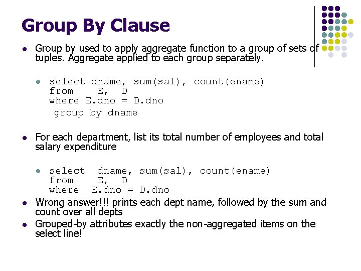
Group By Clause l Group by used to apply aggregate function to a group of sets of tuples. Aggregate applied to each group separately. l select dname, sum(sal), count(ename) from E, D where E. dno = D. dno group by dname l For each department, list its total number of employees and total salary expenditure l select dname, sum(sal), count(ename) from E, D where E. dno = D. dno Wrong answer!!! prints each dept name, followed by the sum and count over all depts Grouped-by attributes exactly the non-aggregated items on the select line! l l

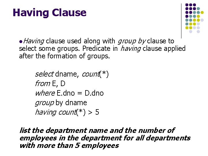
Having Clause l. Having clause used along with group by clause to select some groups. Predicate in having clause applied after the formation of groups. select dname, count(*) from E, D where E. dno = D. dno group by dname having count(*) > 5 list the department name and the number of employees in the department for all departments with more than 5 employees

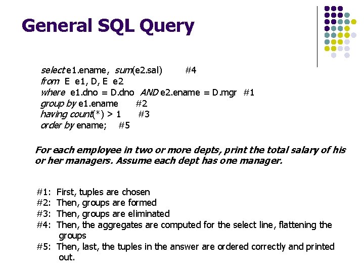
General SQL Query select e 1. ename, sum(e 2. sal) #4 from E e 1, D, E e 2 where e 1. dno = D. dno AND e 2. ename = D. mgr #1 group by e 1. ename #2 having count(*) > 1 #3 order by ename; #5 For each employee in two or more depts, print the total salary of his or her managers. Assume each dept has one manager. #1: #2: #3: #4: First, tuples are chosen Then, groups are formed Then, groups are eliminated Then, the aggregates are computed for the select line, flattening the groups #5: Then, last, the tuples in the answer are ordered correctly and printed out.

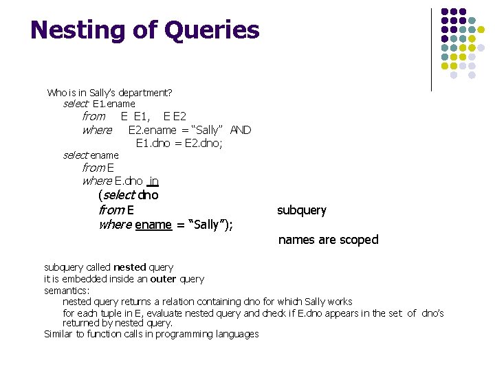
Nesting of Queries Who is in Sally’s department? select E 1. ename from E E 1, E E 2 where E 2. ename = “Sally” AND select ename E 1. dno = E 2. dno; from E where E. dno in (select dno from E where ename = “Sally”); subquery names are scoped subquery called nested query it is embedded inside an outer query semantics: nested query returns a relation containing dno for which Sally works for each tuple in E, evaluate nested query and check if E. dno appears in the set of dno’s returned by nested query. Similar to function calls in programming languages

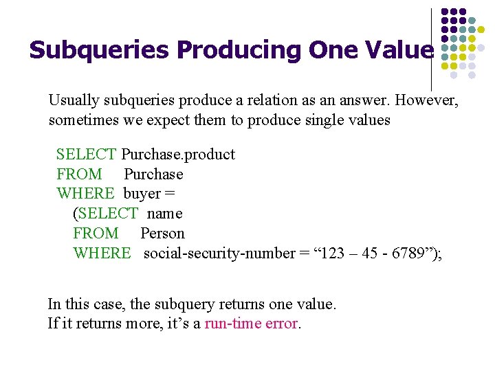
Subqueries Producing One Value Usually subqueries produce a relation as an answer. However, sometimes we expect them to produce single values SELECT Purchase. product FROM Purchase WHERE buyer = (SELECT name FROM Person WHERE social-security-number = “ 123 – 45 - 6789”); In this case, the subquery returns one value. If it returns more, it’s a run-time error.

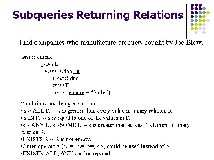
Subqueries Returning Relations Find companies who manufacture products bought by Joe Blow. select ename from E where E. dno in (select dno from E where ename = “Sally”); Conditions involving Relations: • s > ALL R -- s is greater than every value in unary relation R • s IN R -- s is equal to one of the values in R • s > ANY R, s >SOME R -- s is greater than at least 1 element in unary relation R. • EXISTS R -- R is not empty. • Other operators (<, = , <=, >=, <>) could be used instead of >. • EXISTS, ALL, ANY can be negated.

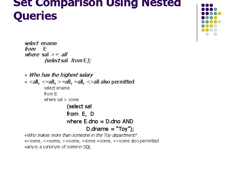
Set Comparison Using Nested Queries select ename from E where sal >= all (select sal from E); l Who has the highest salary l <all, <=all, >=all, <>all also permitted select ename from E where sal > some (select sal from E, D where E. dno = D. dno AND D. dname = “Toy”); l. Who makes more than someone in the Toy department? l<some, <=some, >some =some, <>some also permitted lany is a synonym of some in SQL

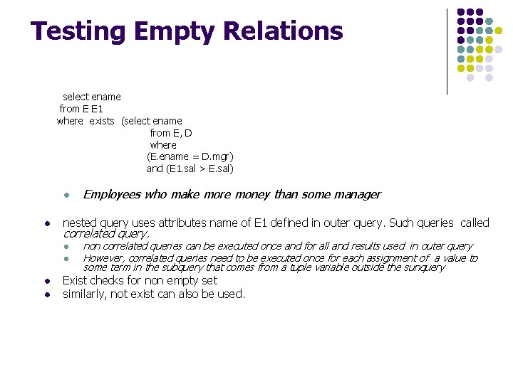
Testing Empty Relations select ename from E E 1 where exists (select ename from E, D where (E. ename = D. mgr) and (E 1. sal > E. sal) l l nested query uses attributes name of E 1 defined in outer query. Such queries called correlated query. l l Employees who make more money than some manager non correlated queries can be executed once and for all and results used in outer query However, correlated queries need to be executed once for each assignment of a value to some term in the subquery that comes from a tuple variable outside the sunquery Exist checks for non empty set similarly, not exist can also be used.

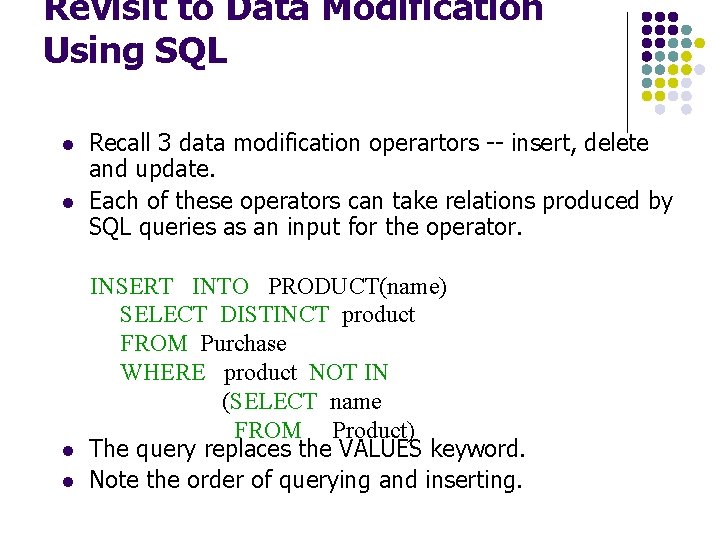
Revisit to Data Modification Using SQL l l Recall 3 data modification operartors -- insert, delete and update. Each of these operators can take relations produced by SQL queries as an input for the operator. INSERT INTO PRODUCT(name) SELECT DISTINCT product FROM Purchase WHERE product NOT IN (SELECT name FROM Product) The query replaces the VALUES keyword. Note the order of querying and inserting.

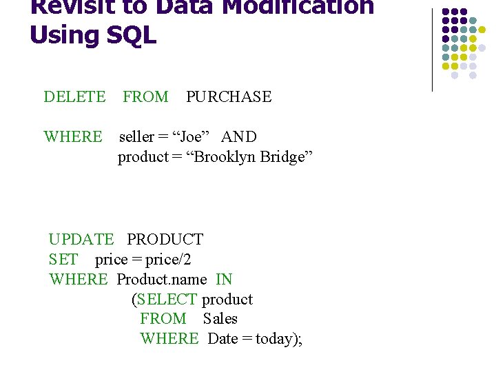
Revisit to Data Modification Using SQL DELETE FROM PURCHASE WHERE seller = “Joe” AND product = “Brooklyn Bridge” UPDATE PRODUCT SET price = price/2 WHERE Product. name IN (SELECT product FROM Sales WHERE Date = today);

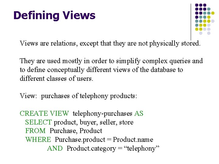
Defining Views are relations, except that they are not physically stored. They are used mostly in order to simplify complex queries and to define conceptually different views of the database to different classes of users. View: purchases of telephony products: CREATE VIEW telephony-purchases AS SELECT product, buyer, seller, store FROM Purchase, Product WHERE Purchase. product = Product. name AND Product. category = “telephony”

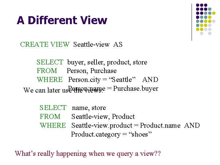
A Different View CREATE VIEW Seattle-view AS SELECT buyer, seller, product, store FROM Person, Purchase WHERE Person. city = “Seattle” AND Person. name We can later use the views: = Purchase. buyer SELECT name, store FROM Seattle-view, Product WHERE Seattle-view. product = Product. name AND Product. category = “shoes” What’s really happening when we query a view? ?

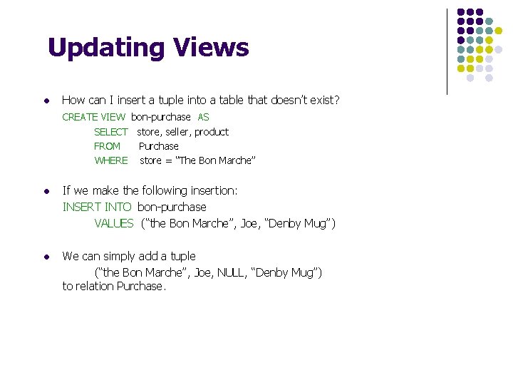
Updating Views l How can I insert a tuple into a table that doesn’t exist? CREATE VIEW bon-purchase AS SELECT store, seller, product FROM Purchase WHERE store = “The Bon Marche” l If we make the following insertion: INSERT INTO bon-purchase VALUES (“the Bon Marche”, Joe, “Denby Mug”) l We can simply add a tuple (“the Bon Marche”, Joe, NULL, “Denby Mug”) to relation Purchase.

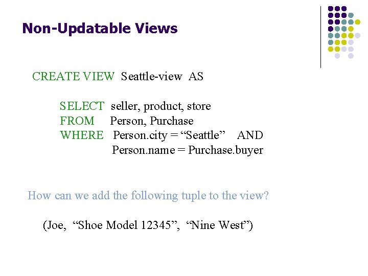
Non-Updatable Views CREATE VIEW Seattle-view AS SELECT seller, product, store FROM Person, Purchase WHERE Person. city = “Seattle” AND Person. name = Purchase. buyer How can we add the following tuple to the view? (Joe, “Shoe Model 12345”, “Nine West”)

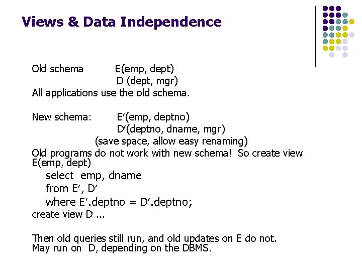
Views & Data Independence Old schema E(emp, dept) D (dept, mgr) All applications use the old schema. New schema: E¢(emp, deptno) D¢(deptno, dname, mgr) (save space, allow easy renaming) Old programs do not work with new schema! So create view E(emp, dept) select emp, dname from E¢, D¢ where E¢. deptno = D¢. deptno; create view D. . . Then old queries still run, and old updates on E do not. May run on D, depending on the DBMS.