Minimizing Average FlowTime Naveen Garg IIT Delhi Joint

Minimizing Average Flow-Time Naveen Garg IIT Delhi Joint work with Amit Kumar, Jivi Chadha , V Muralidhara, S. Anand

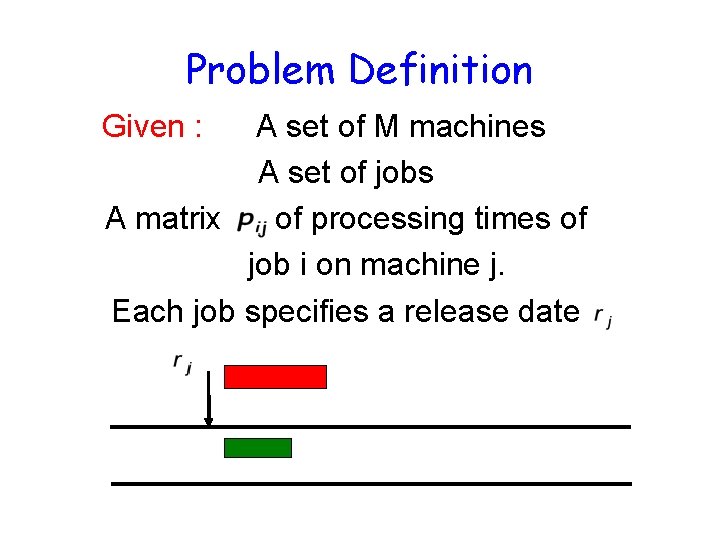
Problem Definition Given : A set of M machines A set of jobs A matrix of processing times of job i on machine j. Each job specifies a release date

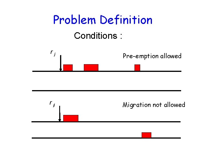
Problem Definition Conditions : Pre-emption allowed Migration not allowed

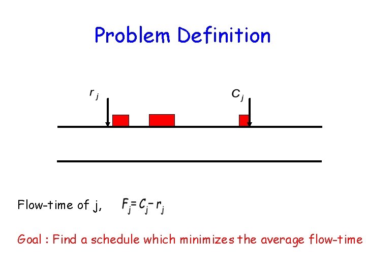
Problem Definition Flow-time of j, Goal : Find a schedule which minimizes the average flow-time

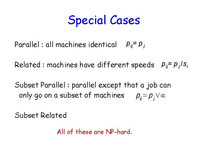
Special Cases Parallel : all machines identical Related : machines have different speeds Subset Parallel : parallel except that a job can only go on a subset of machines Subset Related All of these are NP-hard.

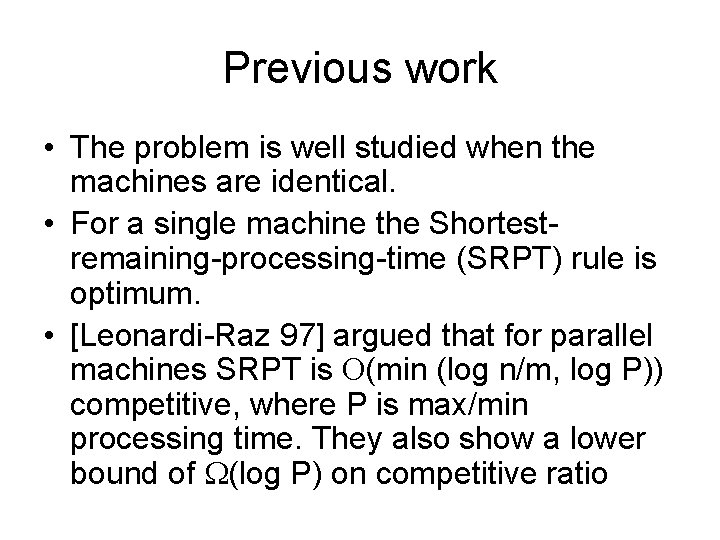
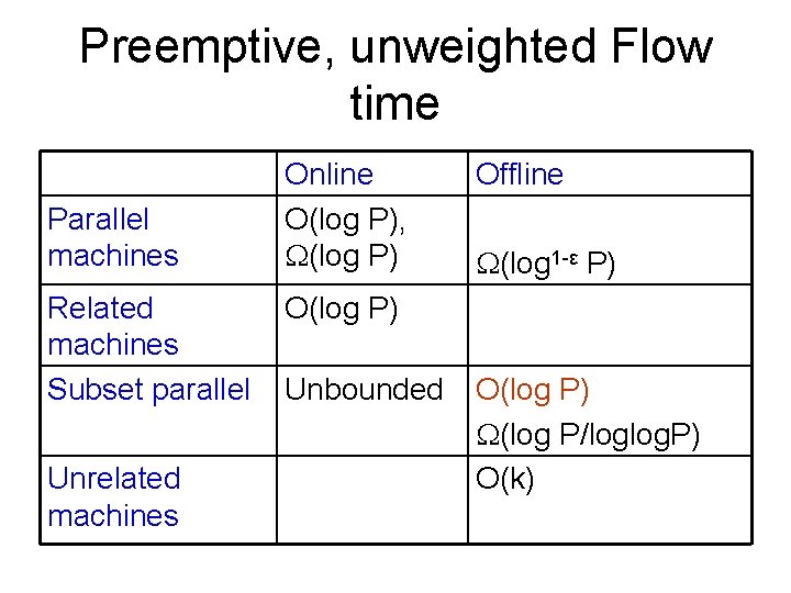
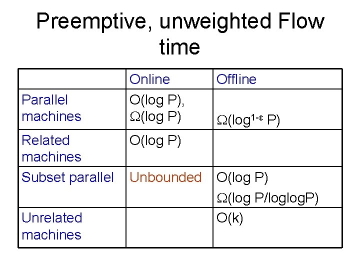
Previous work • The problem is well studied when the machines are identical. • For a single machine the Shortestremaining-processing-time (SRPT) rule is optimum. • [Leonardi-Raz 97] argued that for parallel machines SRPT is O(min (log n/m, log P)) competitive, where P is max/min processing time. They also show a lower bound of (log P) on competitive ratio

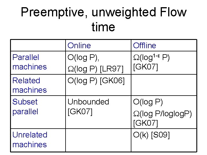
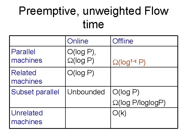
Preemptive, unweighted Flow time Parallel machines Related machines Subset parallel Unrelated machines Online O(log P), (log P) [LR 97] O(log P) [GK 06] Offline (log 1 -ε P) [GK 07] Unbounded [GK 07] O(log P) (log P/loglog. P) [GK 07] O(k) [S 09]

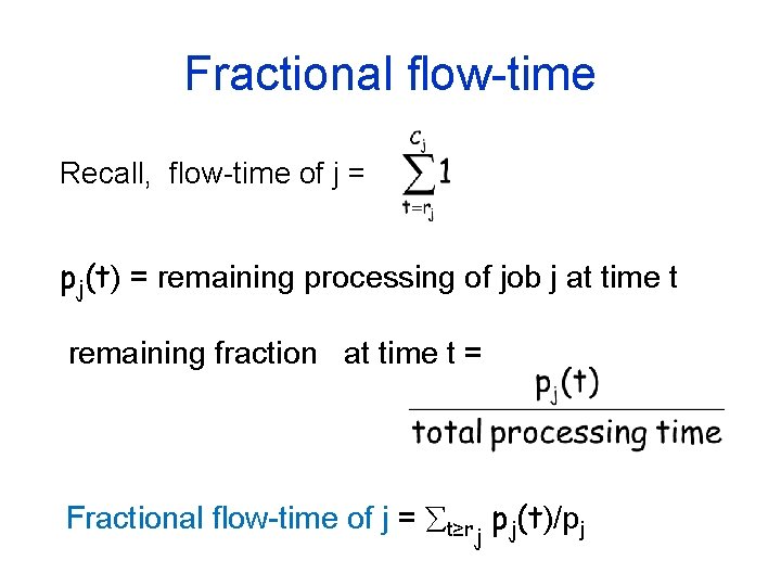
Fractional flow-time Recall, flow-time of j = pj(t) = remaining processing of job j at time t remaining fraction at time t = Fractional flow-time of j = t≥rj pj(t)/pj

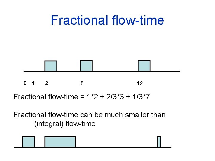
Fractional flow-time 0 1 2 5 12 Fractional flow-time = 1*2 + 2/3*3 + 1/3*7 Fractional flow-time can be much smaller than (integral) flow-time

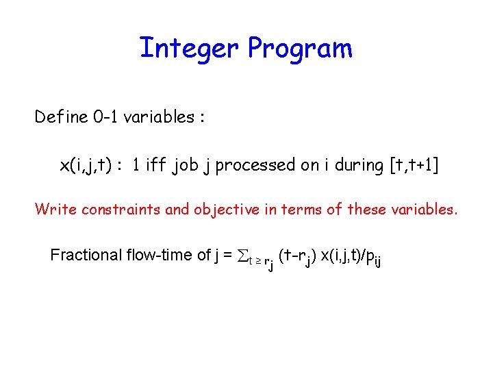
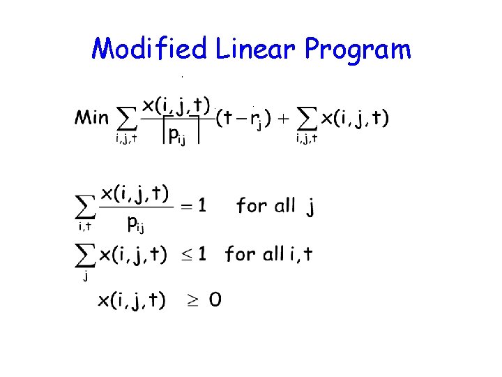
Integer Program Define 0 -1 variables : x(i, j, t) : 1 iff job j processed on i during [t, t+1] Write constraints and objective in terms of these variables. Fractional flow-time of j = t ≥ rj (t-rj) x(i, j, t)/pij

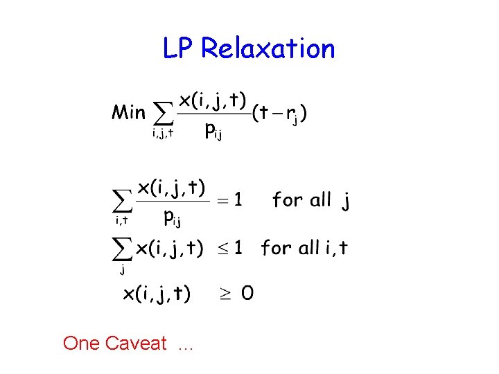
LP Relaxation One Caveat …

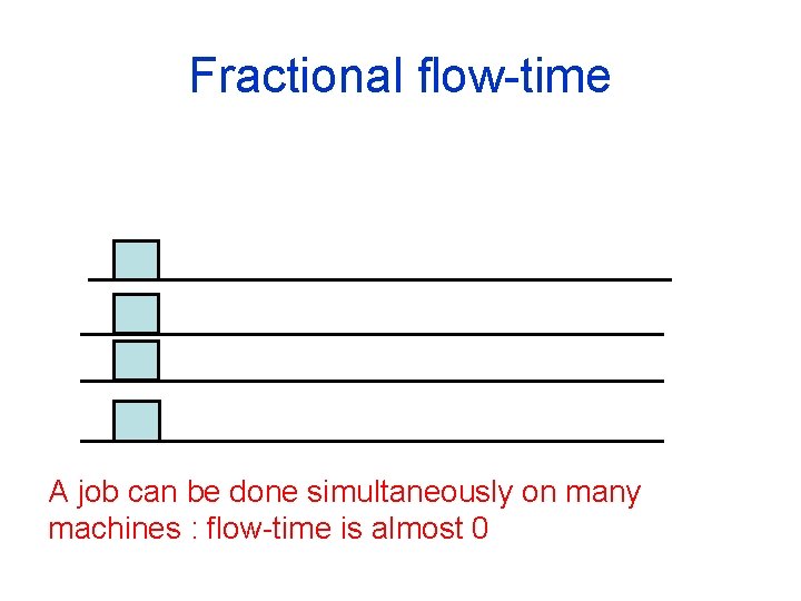
Fractional flow-time A job can be done simultaneously on many machines : flow-time is almost 0

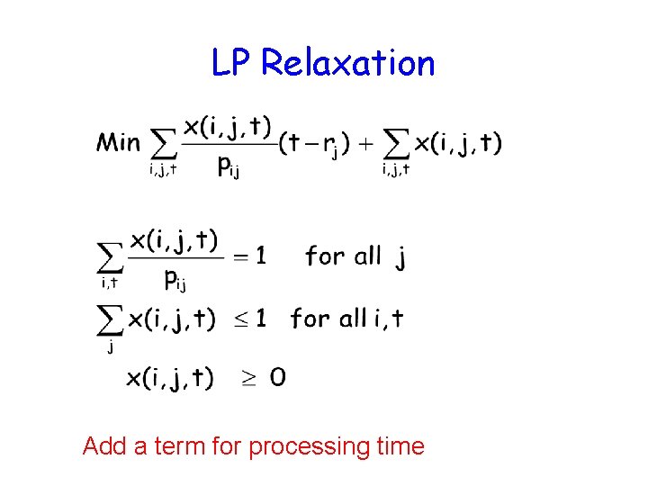
LP Relaxation Add a term for processing time

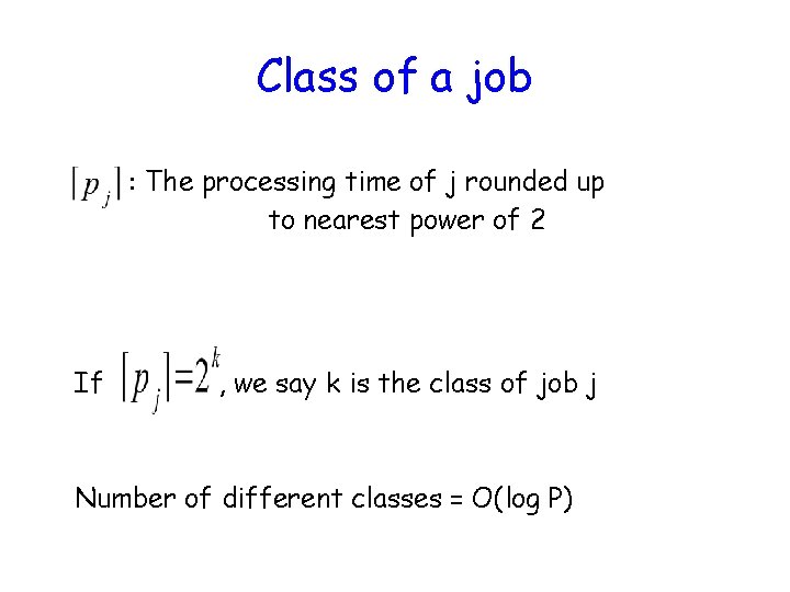
Class of a job : The processing time of j rounded up to nearest power of 2 If , we say k is the class of job j Number of different classes = O(log P)

Modified Linear Program

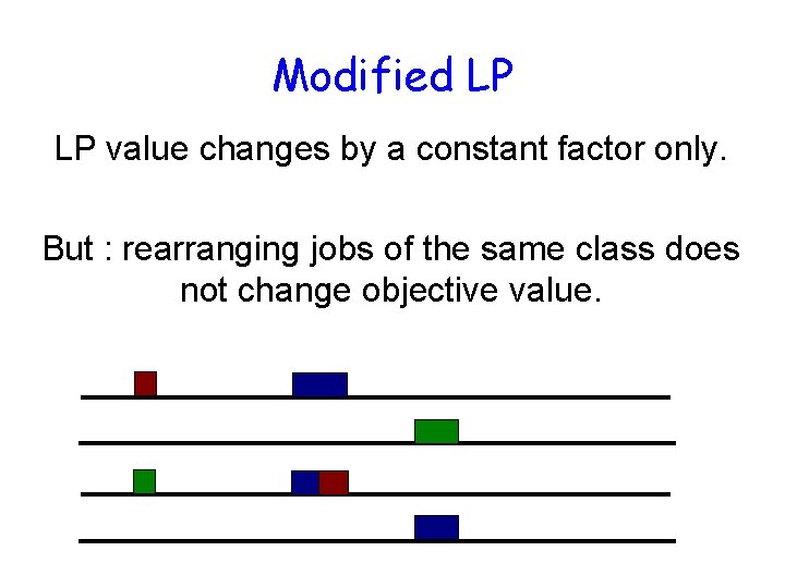
Modified LP LP value changes by a constant factor only. But : rearranging jobs of the same class does not change objective value.

From fractional to integral • The solution to the LP is not feasible for our (integral) problem since it schedules the same job on multiple m/c’s. • We now show to get a feasible, nonmigratory schedule.

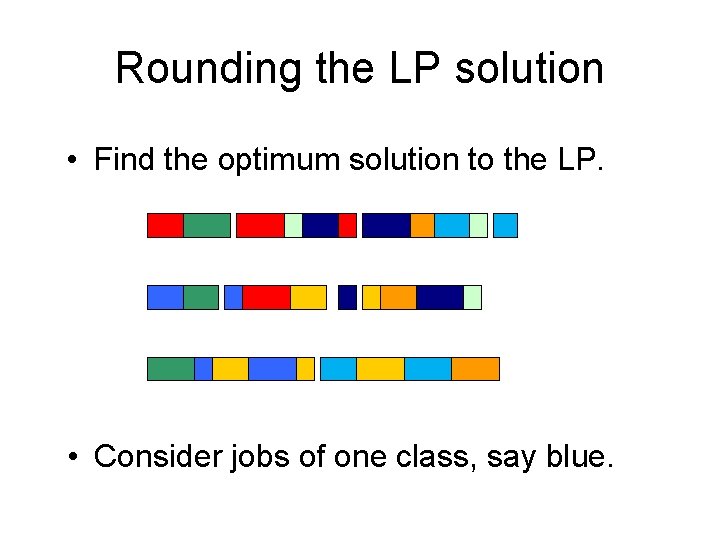
Rounding the LP solution • Find the optimum solution to the LP. • Consider jobs of one class, say blue.

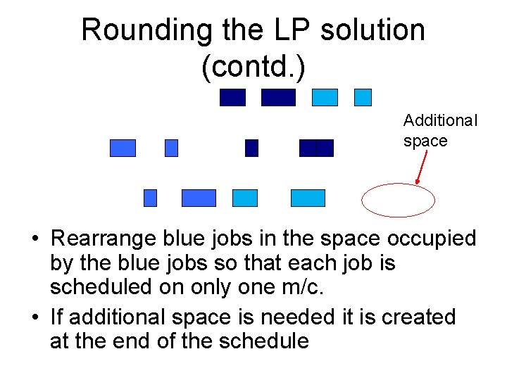
Rounding the LP solution (contd. ) Additional space • Rearrange blue jobs in the space occupied by the blue jobs so that each job is scheduled on only one m/c. • If additional space is needed it is created at the end of the schedule

Preemptive, unweighted Flow time Parallel machines Related machines Subset parallel Unrelated machines Online O(log P), (log P) Offline (log 1 -ε P) O(log P) Unbounded O(log P) (log P/loglog. P) O(k)

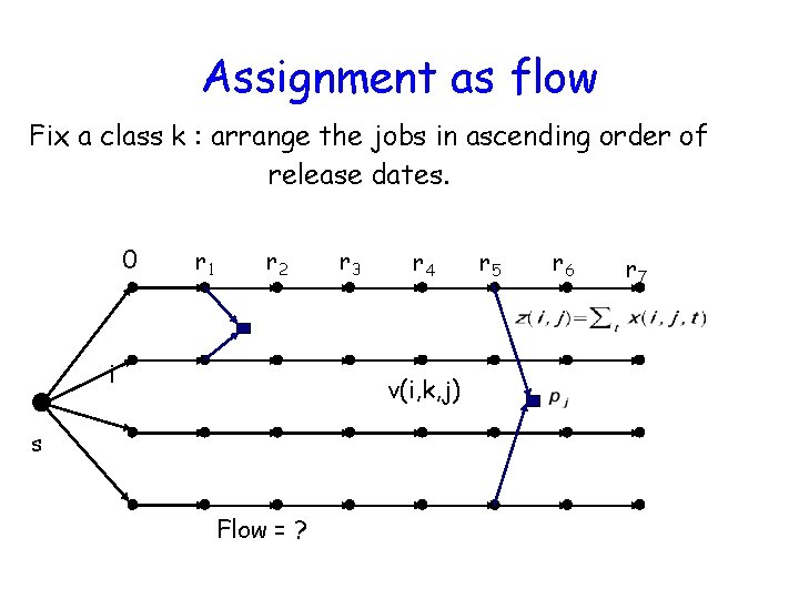
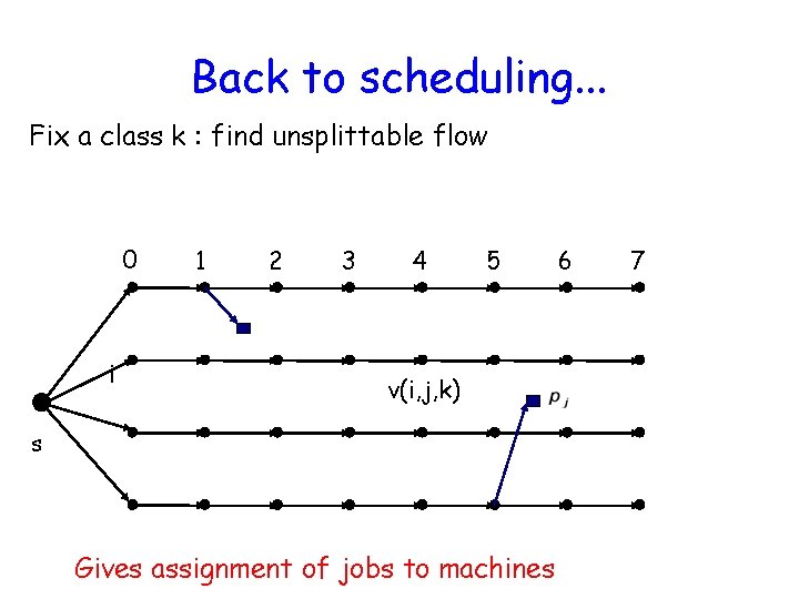
Assignment as flow Fix a class k : arrange the jobs in ascending order of release dates. 0 r 1 r 2 i r 3 r 4 v(i, k, j) s Flow = ? r 5 r 6 r 7

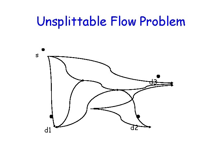
Unsplittable Flow Problem s d 3 d 1 d 2

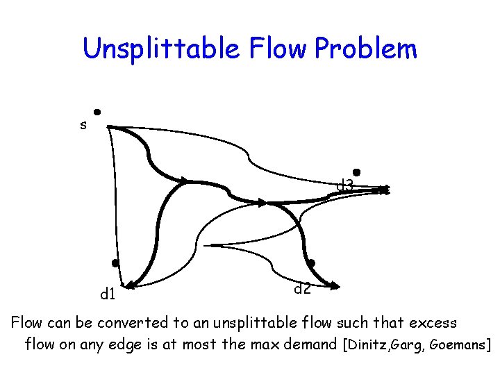
Unsplittable Flow Problem s d 3 d 1 d 2 Flow can be converted to an unsplittable flow such that excess flow on any edge is at most the max demand [Dinitz, Garg, Goemans]

Back to scheduling. . . Fix a class k : find unsplittable flow 0 i 1 2 3 4 5 v(i, j, k) s Gives assignment of jobs to machines 6 7

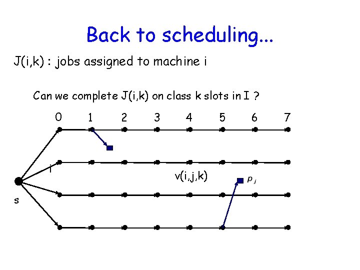
Back to scheduling. . . J(i, k) : jobs assigned to machine i Can we complete J(i, k) on class k slots in I ? 0 i s 1 2 3 4 v(i, j, k) 5 6 7

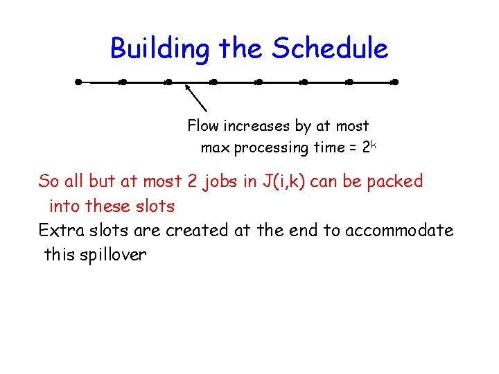
Building the Schedule Flow increases by at most max processing time = 2 k So all but at most 2 jobs in J(i, k) can be packed into these slots Extra slots are created at the end to accommodate this spillover

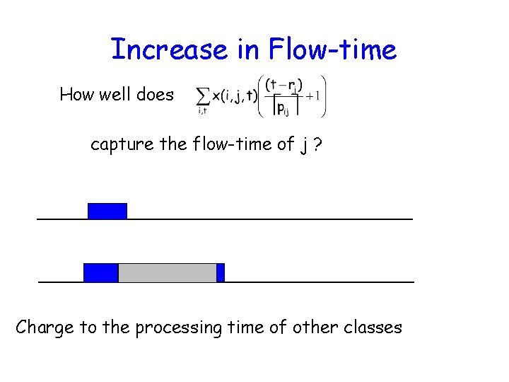
Increase in Flow-time How well does capture the flow-time of j ? Charge to the processing time of other classes

Finally. . . Since there are only log P classes… Can get OPT + O(log P). processing time flow-time for subset parallel case.

Preemptive, unweighted Flow time Parallel machines Related machines Subset parallel Unrelated machines Online O(log P), (log P) Offline (log 1 -ε P) O(log P) Unbounded O(log P) (log P/loglog. P) O(k)

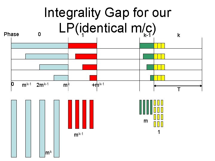
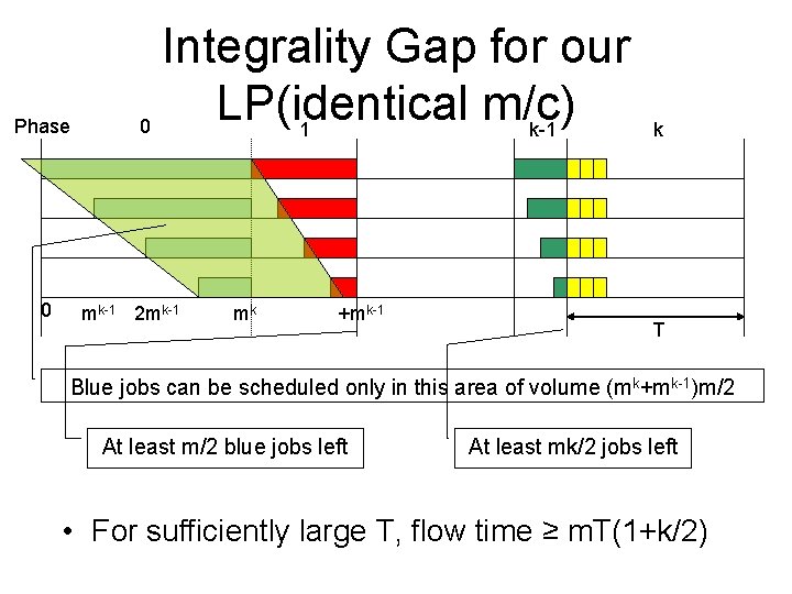
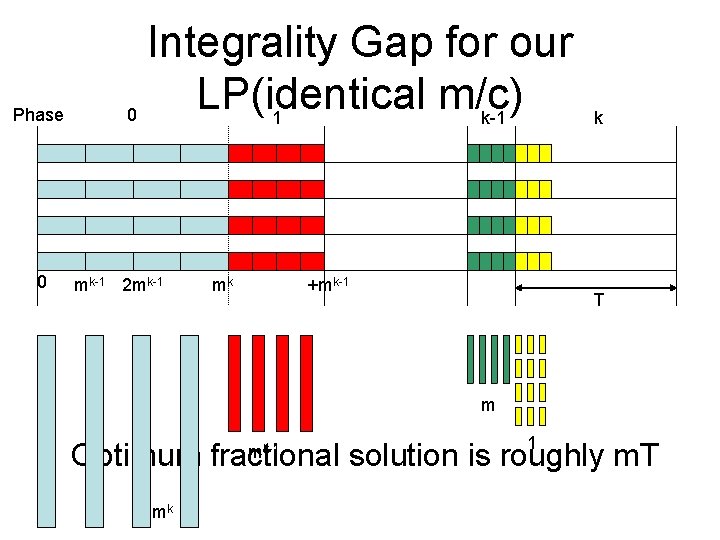
Phase 0 Integrality Gap for our LP(identical m/c) 0 1 k-1 mk-1 2 mk-1 mk +mk-1 T m mk-1 mk k 1

Phase 0 Integrality Gap for our LP(identical m/c) 0 1 k-1 mk-1 2 mk-1 mk +mk-1 k T Blue jobs can be scheduled only in this area of volume (mk+mk-1)m/2 At least m/2 blue jobs left At least mk/2 jobs left • For sufficiently large T, flow time ≥ m. T(1+k/2)

Phase 0 Integrality Gap for our LP(identical m/c) 0 1 k-1 mk-1 2 mk-1 mk +mk-1 k T m 1 • Optimum fractional solution is roughly m. T mk-1 mk

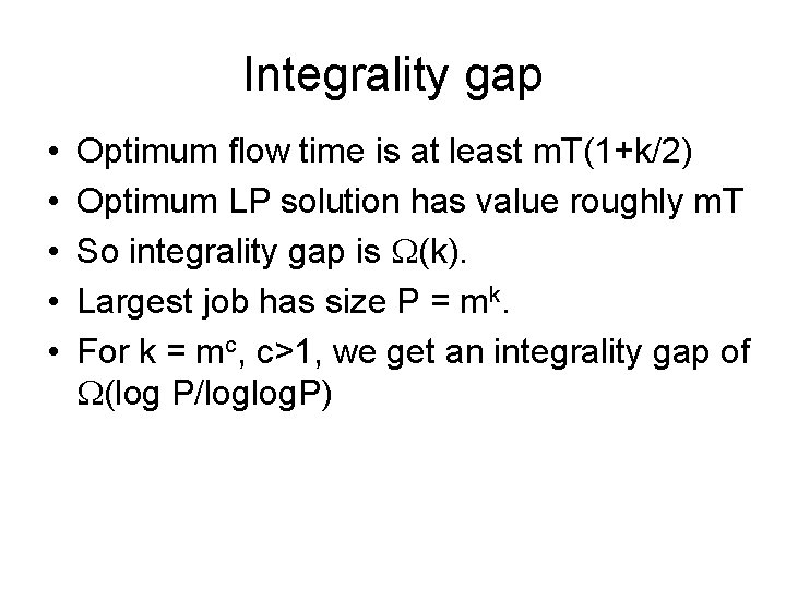
Integrality gap • • • Optimum flow time is at least m. T(1+k/2) Optimum LP solution has value roughly m. T So integrality gap is (k). Largest job has size P = mk. For k = mc, c>1, we get an integrality gap of (log P/loglog. P)

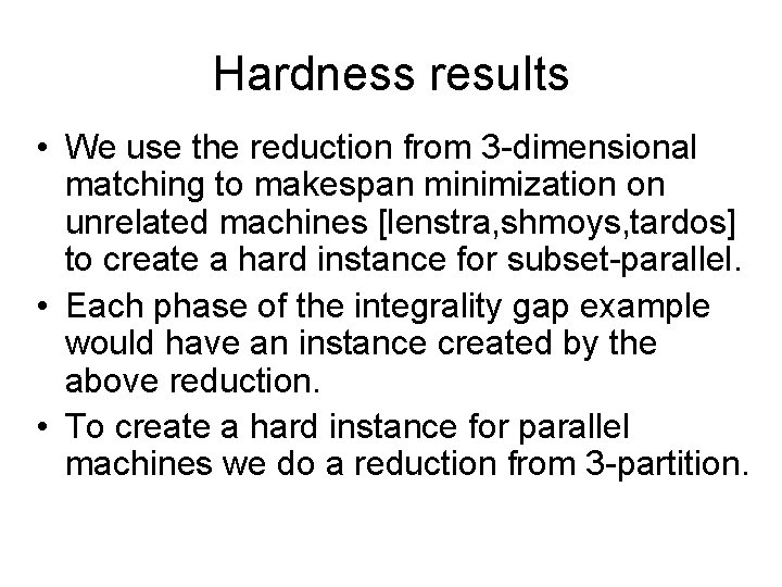
Hardness results • We use the reduction from 3 -dimensional matching to makespan minimization on unrelated machines [lenstra, shmoys, tardos] to create a hard instance for subset-parallel. • Each phase of the integrality gap example would have an instance created by the above reduction. • To create a hard instance for parallel machines we do a reduction from 3 -partition.

Preemptive, unweighted Flow time Parallel machines Related machines Subset parallel Unrelated machines Online O(log P), (log P) Offline (log 1 -ε P) O(log P) Unbounded O(log P) (log P/loglog. P) O(k)

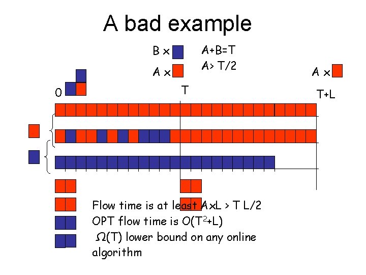
A bad example A+B=T A> T/2 Bx Ax 0 T Flow time is at least Ax. L > T L/2 OPT flow time is O(T 2+L) Ω(T) lower bound on any online algorithm Ax T+L

Other Models • What if we allow the algorithm extra resources ? • In particular, suppose the algorithm can process (1+ε) units in 1 time-unit. [first proposed by Kalyanasundaram, Pruhs 95] Resource Augmentation Model

Resource Augmentation • For a single machine, many natural scheduling algorithms are O(1/e. O(1))competitive with respect to any Lp norm [Bansal Pruhs ‘ 03] • Parallel machines : randomly assign each job to a machine – O(1/e. O(1)) competitive [Chekuri, Goel, Khanna, Kumar ’ 04] • Unrelated Machines : O(1/e 2)-competitive, even for weighted case. [Chadha, Garg, Kumar, Muralidhara ‘ 09]

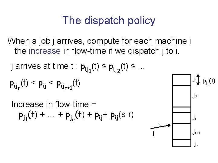
Our Algorithm When a job arrives, we dispatch it to one of the machines. Each machine just follows the optimal policy : Shortest Remaining Processing Time (SRPT) What is the dispatch policy ? GREEDY

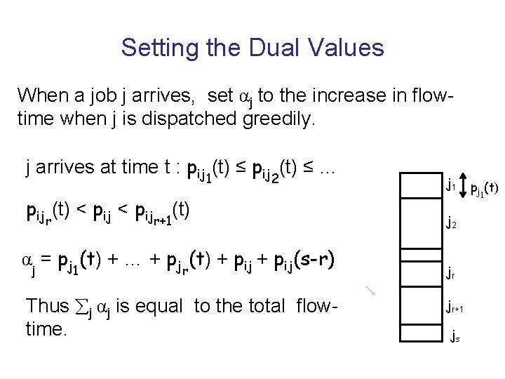
The dispatch policy When a job j arrives, compute for each machine i the increase in flow-time if we dispatch j to i. j arrives at time t : pij 1(t) ≤ pij 2(t) ≤ … j 1 pijr(t) < pijr+1(t) j 2 Increase in flow-time = pj 1(t) + … + pjr(t) + pij(s-r) jr j jr+1 js pj 1(t)

Our Algorithm When a job j arrives, compute for each machine i the increase in flow-time if we dispatch j to i. Dispatch j to the machine for which increase in fractional flow-time is minimum.

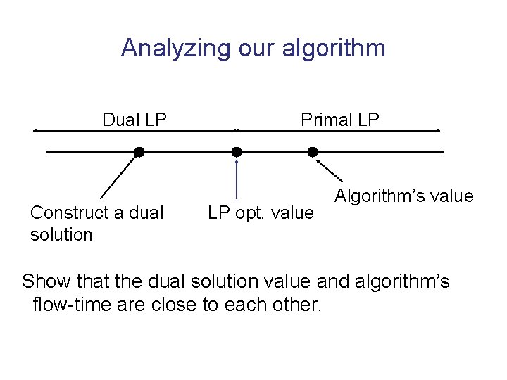
Analyzing our algorithm Dual LP Construct a dual solution Primal LP LP opt. value Algorithm’s value Show that the dual solution value and algorithm’s flow-time are close to each other.

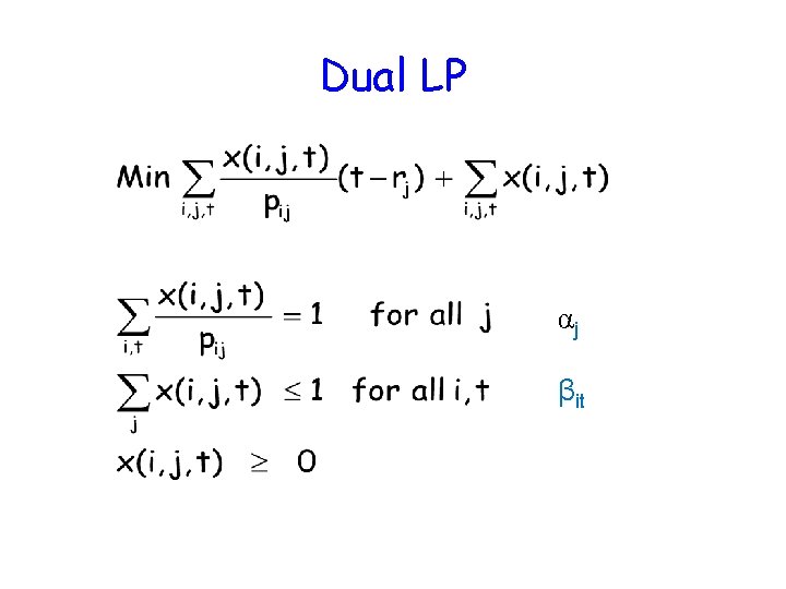
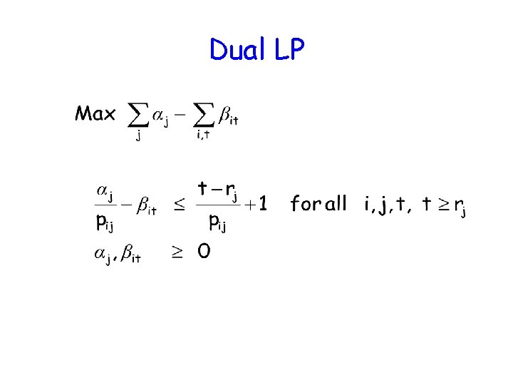
Dual LP αj βit

Dual LP

Setting the Dual Values When a job j arrives, set αj to the increase in flowtime when j is dispatched greedily. j arrives at time t : pij 1(t) ≤ pij 2(t) ≤ … j 1 pijr(t) < pijr+1(t) j 2 αj = pj 1(t) + … + pjr(t) + pij(s-r) Thus j αj is equal to the total flowtime. jr jr+1 js pj 1(t)

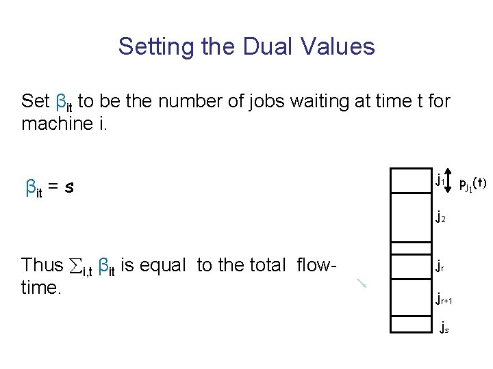
Setting the Dual Values Set βit to be the number of jobs waiting at time t for machine i. βit = s j 1 j 2 Thus i, t βit is equal to the total flowtime. jr jr+1 js pj 1(t)

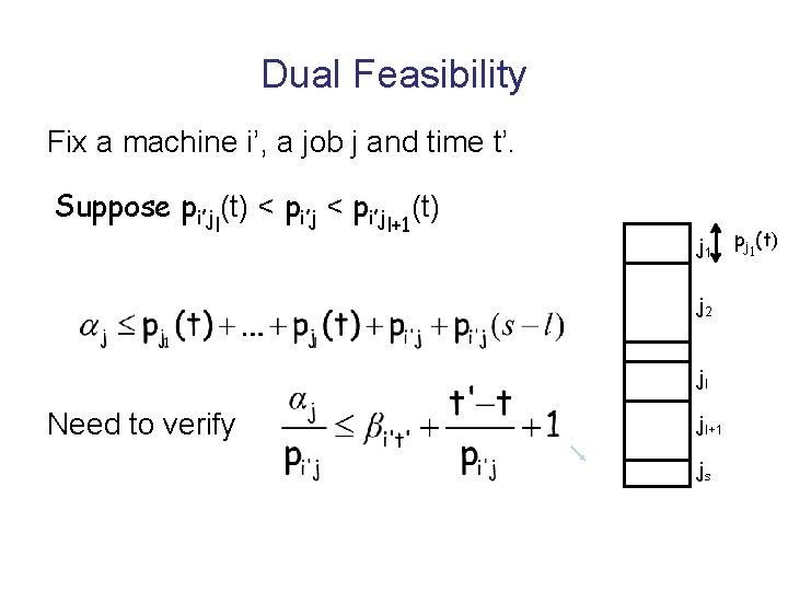
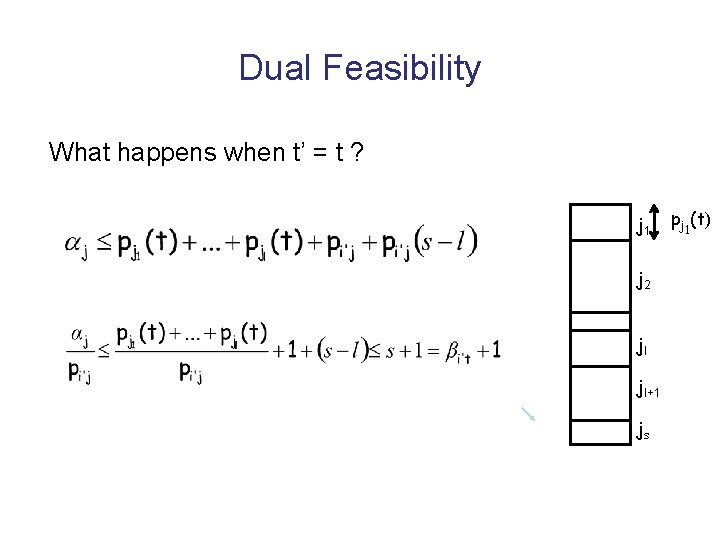
Dual Feasibility Fix a machine i’, a job j and time t’. Suppose pi’jl(t) < pi’jl+1(t) j 1 j 2 jl Need to verify jl+1 js pj 1(t)

Dual Feasibility What happens when t’ = t ? j 1 j 2 jl jl+1 js pj 1(t)

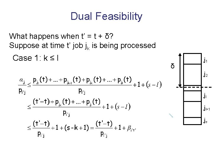
Dual Feasibility What happens when t’ = t + δ? Suppose at time t’ job jk is being processed Case 1: k ≤ l δ j 1 j 2 jl jl+1 js

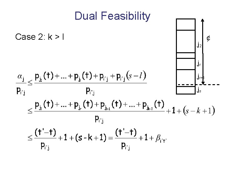
Dual Feasibility Case 2: k > l j 2 jr jr+1 js ¢

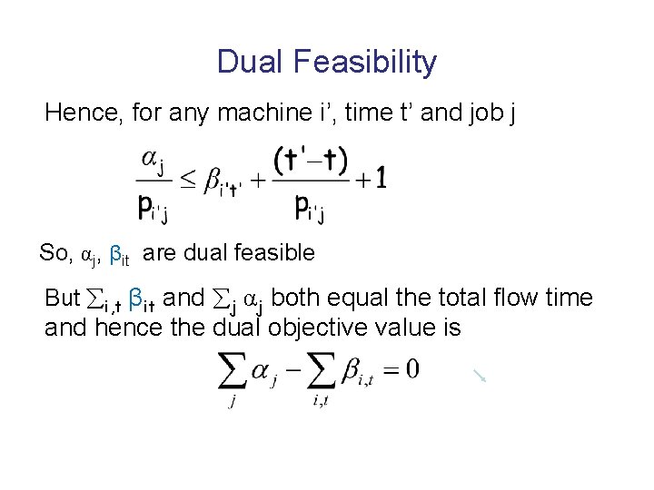
Dual Feasibility Hence, for any machine i’, time t’ and job j So, αj, βit are dual feasible But i, t βit and j αj both equal the total flow time and hence the dual objective value is

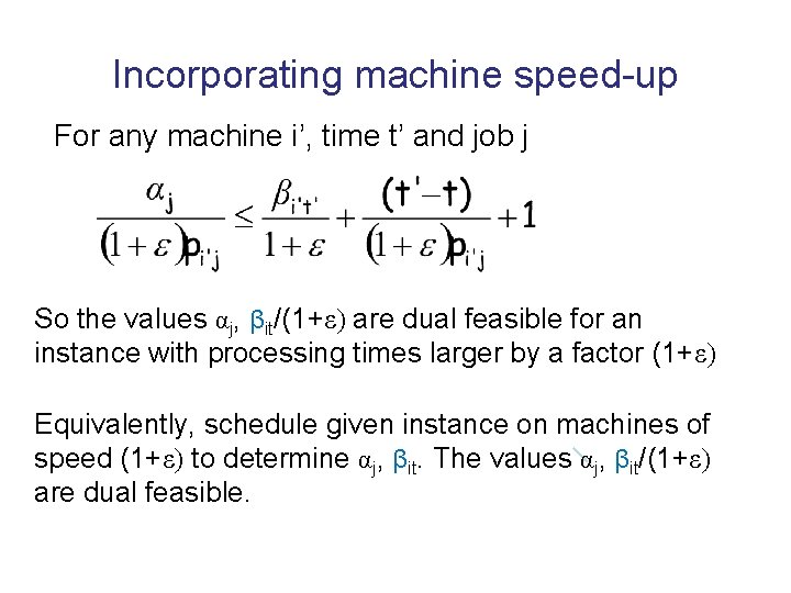
Incorporating machine speed-up For any machine i’, time t’ and job j So the values αj, βit/(1+ε) are dual feasible for an instance with processing times larger by a factor (1+ε) Equivalently, schedule given instance on machines of speed (1+ε) to determine αj, βit. The values αj, βit/(1+ε) are dual feasible.

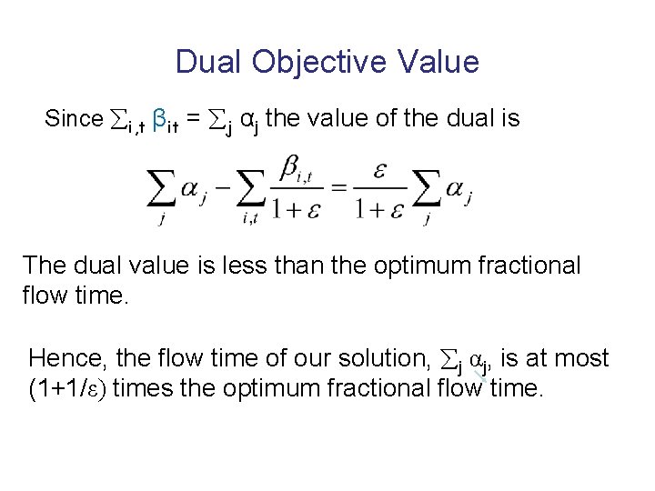
Dual Objective Value Since i, t βit = j αj the value of the dual is The dual value is less than the optimum fractional flow time. Hence, the flow time of our solution, j αj, is at most (1+1/ε) times the optimum fractional flow time.

Extensions • Can extend this analysis to the Lp-norm of the flow time to get a similar result. • Analysis also extends to the case of minimizing sum of flow time and energy on unrelated machines.

Open Problems Single Machine : Constant factor approximation algorithm for weighted flow-time. loglog n approx [Bansal Pruhs ’ 10] 2+ε quasi polynomial time algorithm [Chekuri Khanna Zhu ‘ 01]

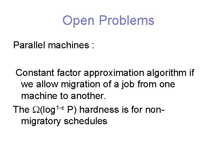
Open Problems Parallel machines : Constant factor approximation algorithm if we allow migration of a job from one machine to another. The (log 1 -ε P) hardness is for nonmigratory schedules

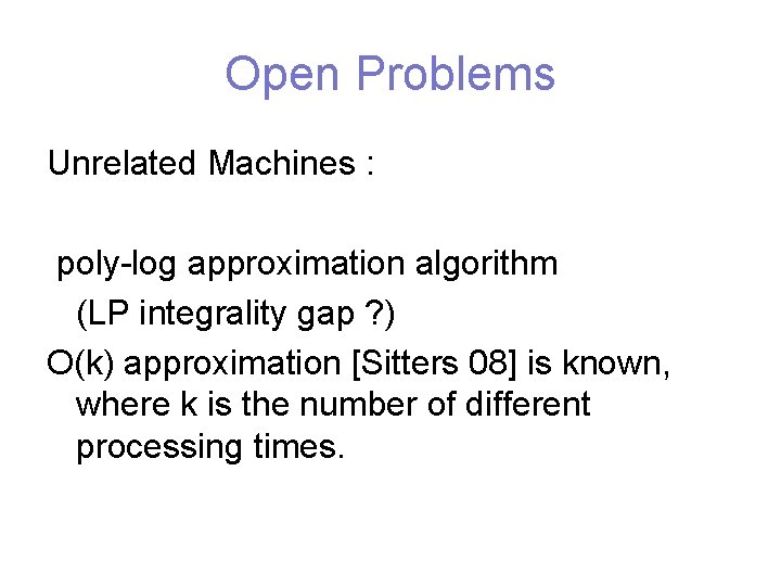
Open Problems Unrelated Machines : poly-log approximation algorithm (LP integrality gap ? ) O(k) approximation [Sitters 08] is known, where k is the number of different processing times.

Thank You