Single Factor ANOVA 2010 Pearson Prentice Hall All

Single Factor ANOVA © 2010 Pearson Prentice Hall. All rights reserved

Analysis of Variance (ANOVA) is an inferential method used to test the equality of three or more population means. 13 -2

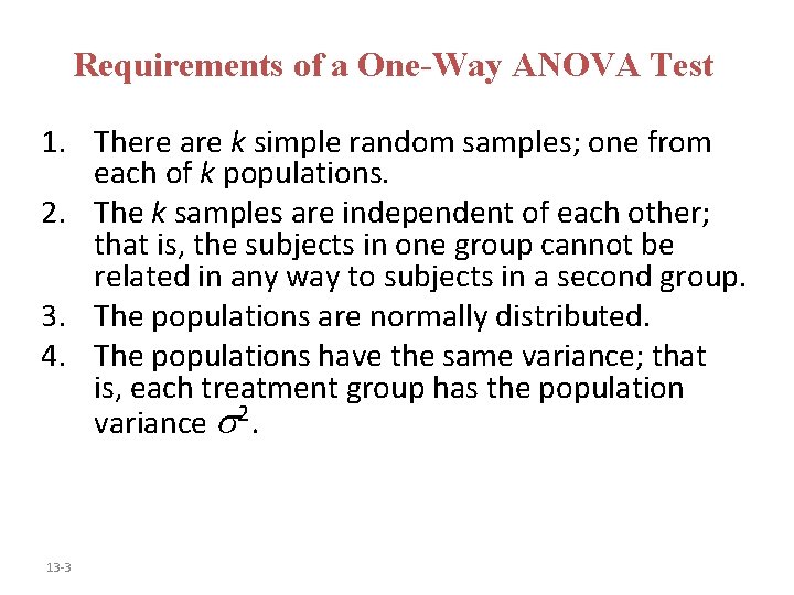
Requirements of a One-Way ANOVA Test 1. There are k simple random samples; one from each of k populations. 2. The k samples are independent of each other; that is, the subjects in one group cannot be related in any way to subjects in a second group. 3. The populations are normally distributed. 4. The populations have the same variance; that is, each treatment group has the population variance 2. 13 -3

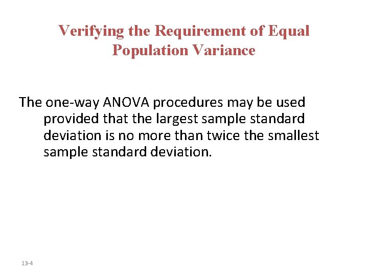
Verifying the Requirement of Equal Population Variance The one-way ANOVA procedures may be used provided that the largest sample standard deviation is no more than twice the smallest sample standard deviation. 13 -4

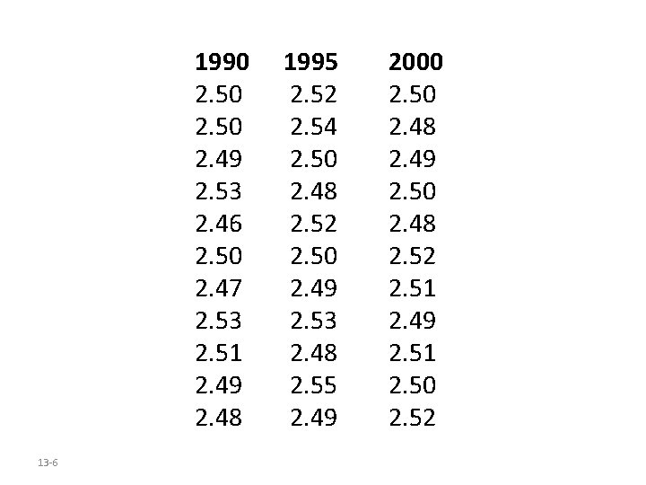
Parallel Example 1: Verifying the Requirements of ANOVA The following data represent the weight (in grams) of pennies minted at the Denver mint in 1990, 1995, and 2000. Verify that the requirements in order to perform a one-way ANOVA are satisfied. 13 -5

1990 2. 50 2. 49 2. 53 2. 46 2. 50 2. 47 2. 53 2. 51 2. 49 2. 48 13 -6 1995 2. 52 2. 54 2. 50 2. 48 2. 52 2. 50 2. 49 2. 53 2. 48 2. 55 2. 49 2000 2. 50 2. 48 2. 49 2. 50 2. 48 2. 52 2. 51 2. 49 2. 51 2. 50 2. 52

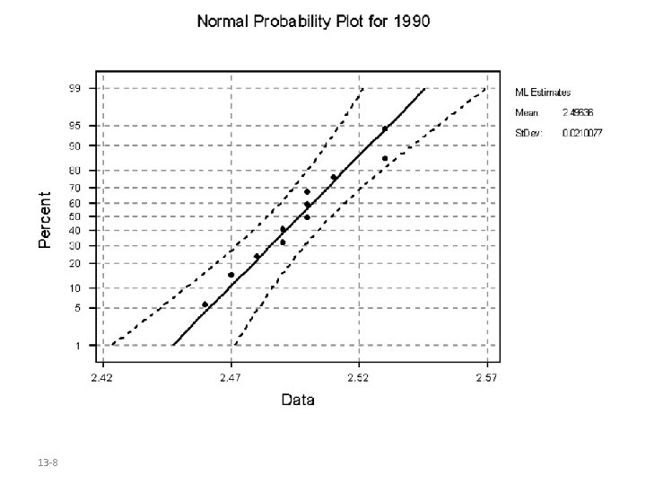
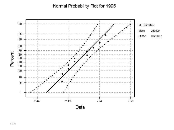
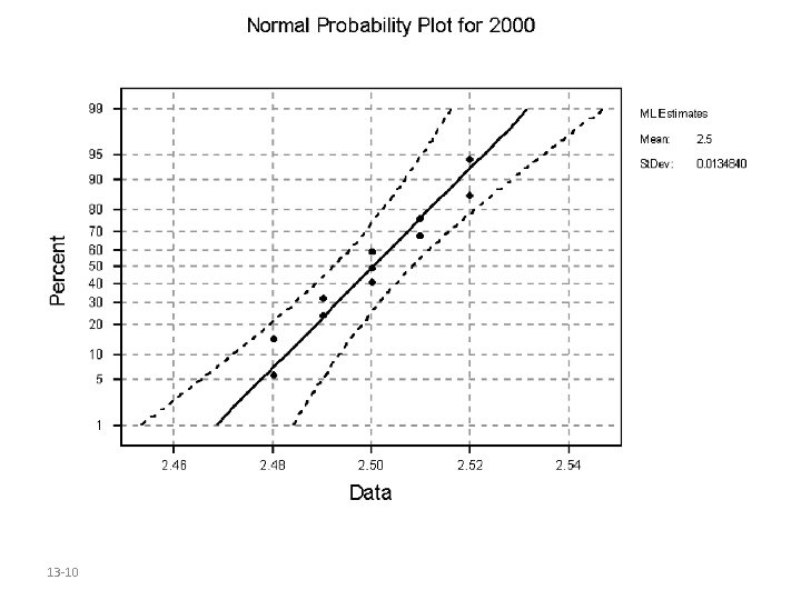
Solution 1. The 3 samples are simple random samples. 2. The samples were obtained independently. 3. Normal probability plots for the 3 years follow. All of the plots are roughly linear so the normality assumption is satisfied. 13 -7

13 -8

13 -9

13 -10

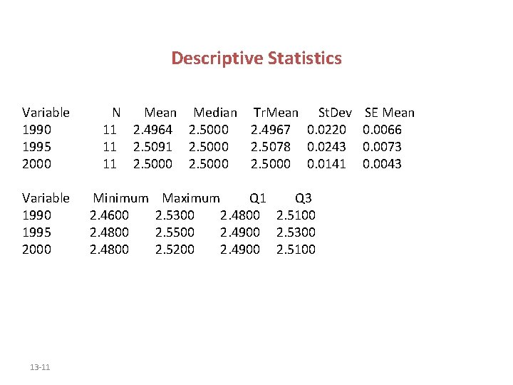
Descriptive Statistics Variable 1990 1995 2000 13 -11 N Mean Median Tr. Mean St. Dev 11 2. 4964 2. 5000 2. 4967 0. 0220 11 2. 5091 2. 5000 2. 5078 0. 0243 11 2. 5000 0. 0141 Minimum 2. 4600 2. 4800 Maximum Q 1 Q 3 2. 5300 2. 4800 2. 5100 2. 5500 2. 4900 2. 5300 2. 5200 2. 4900 2. 5100 SE Mean 0. 0066 0. 0073 0. 0043

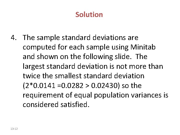
Solution 4. The sample standard deviations are computed for each sample using Minitab and shown on the following slide. The largest standard deviation is not more than twice the smallest standard deviation (2*0. 0141 =0. 0282 > 0. 02430) so the requirement of equal population variances is considered satisfied. 13 -12

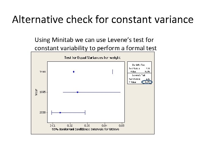
Alternative check for constant variance Using Minitab we can use Levene’s test for constant variability to perform a formal test

The result of Levene’s test shows that there is insufficient evidence to support the claim of nonconstant variability between the populations of interest.

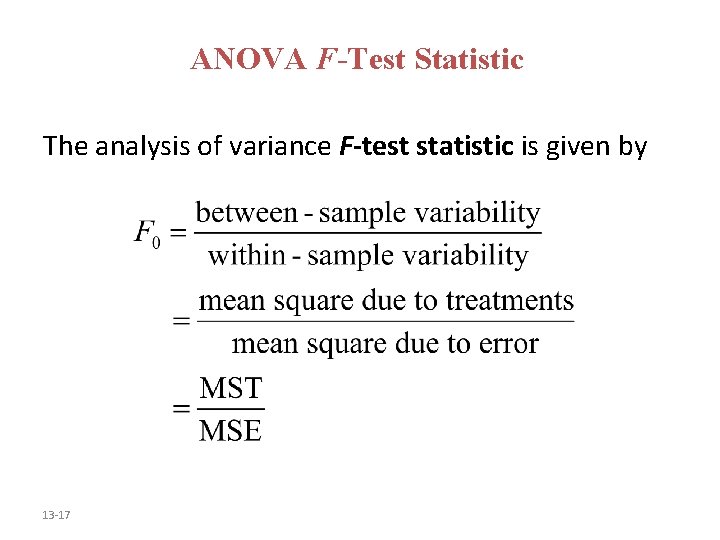
The basic idea in one-way ANOVA is to determine if the sample data could come from populations with the same mean, , or if the sample evidence suggests that at least one sample comes from a population whose mean is different from the others. To make this decision, we compare the variability among the sample means to the variability within each sample. 13 -15

We call the variability among the sample means the between-sample variability, and the variability of each sample the within-sample variability. If the between-sample variability is large relative to the within-sample variability, we have evidence to suggest that the samples come from populations with different means. 13 -16

ANOVA F-Test Statistic The analysis of variance F-test statistic is given by 13 -17

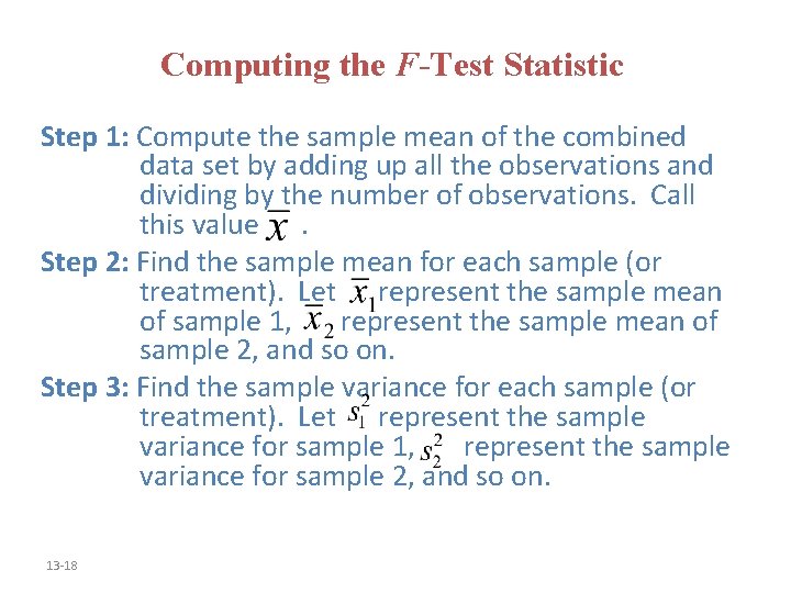
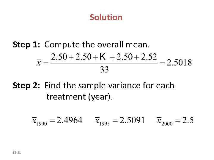
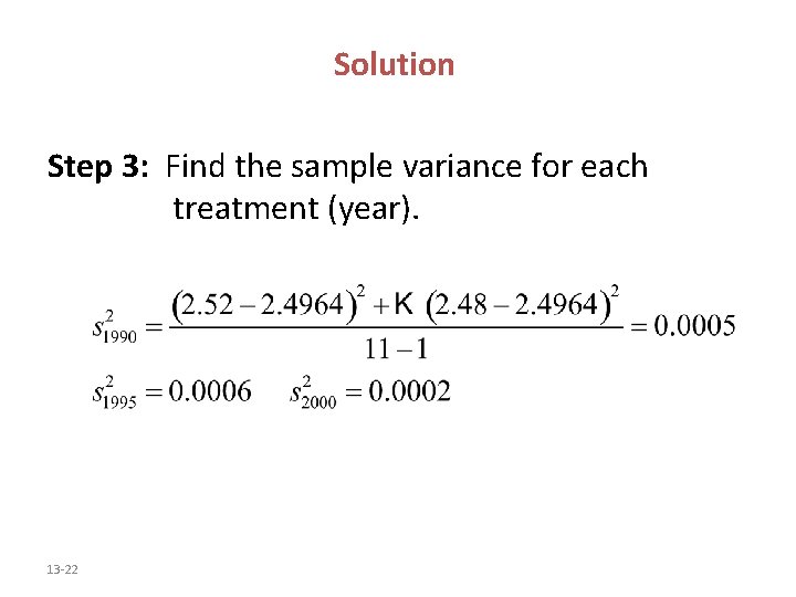
Computing the F-Test Statistic Step 1: Compute the sample mean of the combined data set by adding up all the observations and dividing by the number of observations. Call this value. Step 2: Find the sample mean for each sample (or treatment). Let represent the sample mean of sample 1, represent the sample mean of sample 2, and so on. Step 3: Find the sample variance for each sample (or treatment). Let represent the sample variance for sample 1, represent the sample variance for sample 2, and so on. 13 -18

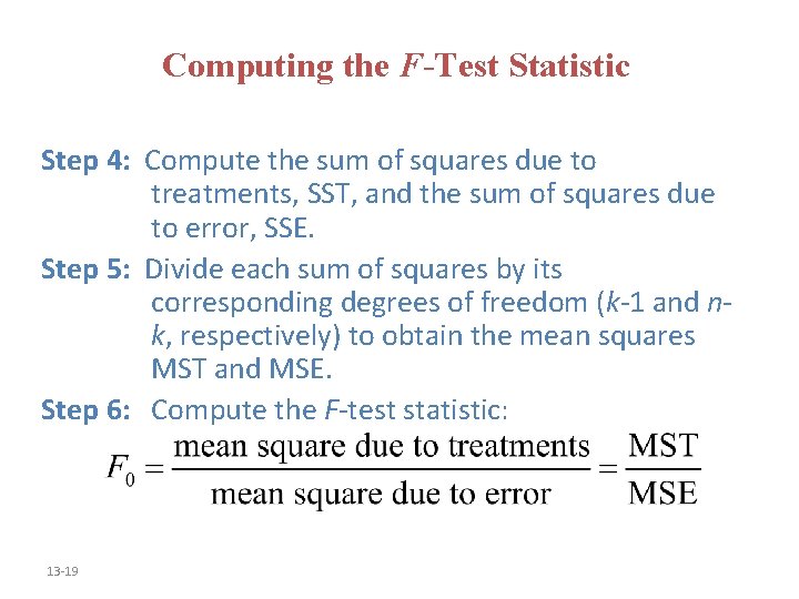
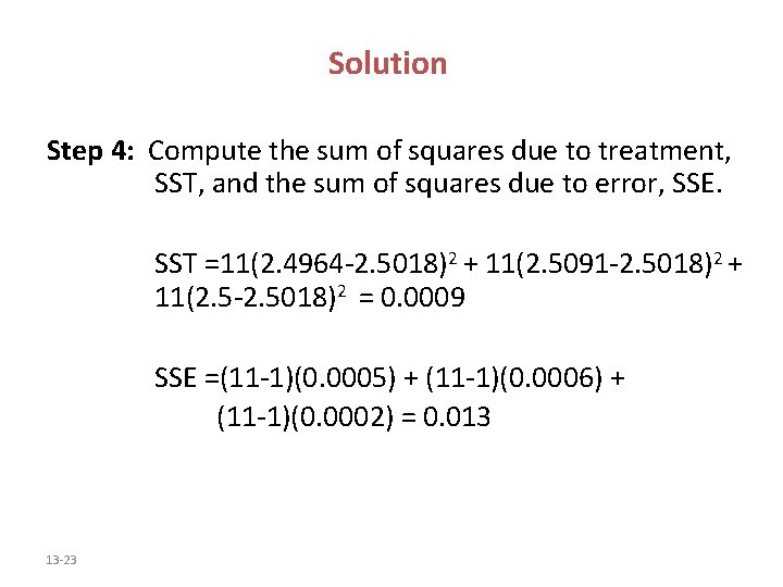
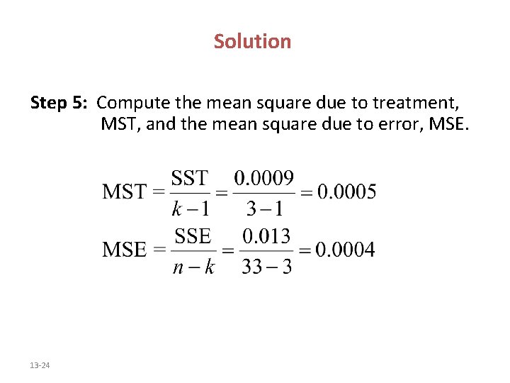
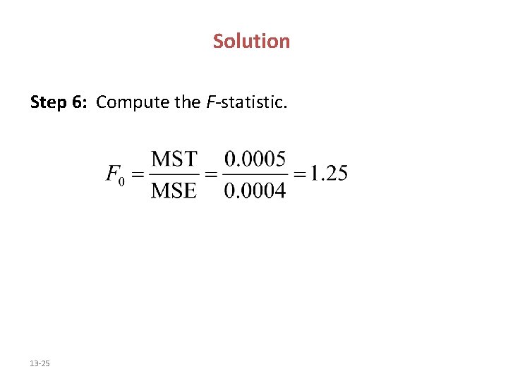
Computing the F-Test Statistic Step 4: Compute the sum of squares due to treatments, SST, and the sum of squares due to error, SSE. Step 5: Divide each sum of squares by its corresponding degrees of freedom (k-1 and nk, respectively) to obtain the mean squares MST and MSE. Step 6: Compute the F-test statistic: 13 -19

Parallel Example 2: Computing the F-Test Statistic Compute the F-test statistic for the penny data. 13 -20

Solution Step 1: Compute the overall mean. Step 2: Find the sample variance for each treatment (year). 13 -21

Solution Step 3: Find the sample variance for each treatment (year). 13 -22

Solution Step 4: Compute the sum of squares due to treatment, SST, and the sum of squares due to error, SSE. SST =11(2. 4964 -2. 5018)2 + 11(2. 5091 -2. 5018)2 + 11(2. 5 -2. 5018)2 = 0. 0009 SSE =(11 -1)(0. 0005) + (11 -1)(0. 0006) + (11 -1)(0. 0002) = 0. 013 13 -23

Solution Step 5: Compute the mean square due to treatment, MST, and the mean square due to error, MSE. 13 -24

Solution Step 6: Compute the F-statistic. 13 -25

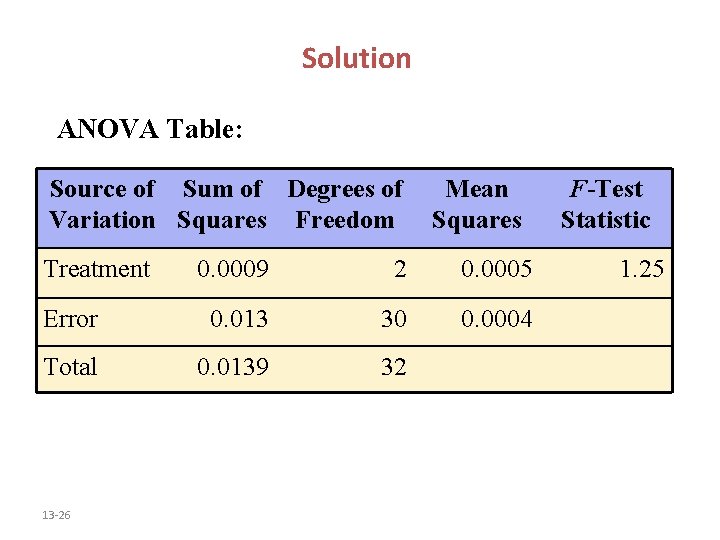
Solution ANOVA Table: Source of Sum of Degrees of Variation Squares Freedom Treatment Mean Squares 0. 0009 2 0. 0005 Error 0. 013 30 0. 0004 Total 0. 0139 32 13 -26 F-Test Statistic 1. 25

Decision Rule in the One-Way ANOVA Test If the P-value is less than the level of significance, , reject the null hypothesis. 13 -27

For the pennies data a F-statistic of 1. 25 results in a P-value of 0. 301. Since the P-value exceeds the default level of significance of 0. 05 we will fail to reject H 0. Conclusion: We have insufficient evidence at the 5% level of significance to support the claim that the mean weight of pennies for at least one of the years does not equal the others.