CHAPTER 12 Statistics 2010 Pearson Prentice Hall All

CHAPTER 12 Statistics © 2010 Pearson Prentice Hall. All rights reserved.

12. 4 The Normal Distribution © 2010 Pearson Prentice Hall. All rights reserved. 2

1. 2. 3. 4. 5. Objectives Recognize characteristics of normal distributions. Understand the 68 -95 -99. 7 Rule. Find scores at a specified number of standard deviations from the mean. Use the 68 -95 -99. 7 Rule Convert a data item to a z-score. 6. Understand percentiles and quartiles. 7. Use and interpret margins of error. 8. Recognize distributions that are not normal. © 2010 Pearson Prentice Hall. All rights reserved. 3

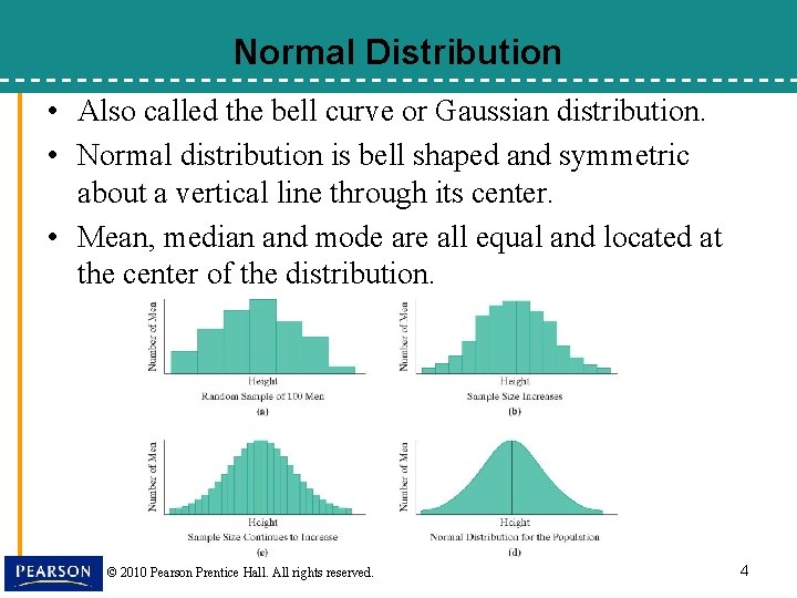
Normal Distribution • Also called the bell curve or Gaussian distribution. • Normal distribution is bell shaped and symmetric about a vertical line through its center. • Mean, median and mode are all equal and located at the center of the distribution. © 2010 Pearson Prentice Hall. All rights reserved. 4

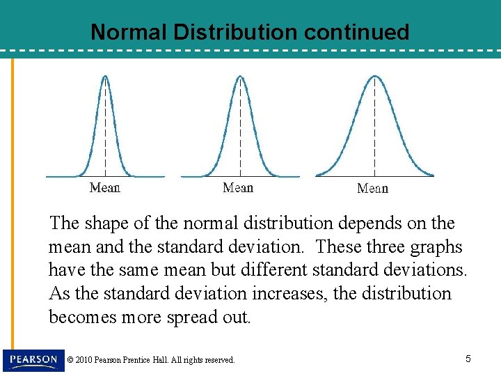
Normal Distribution continued The shape of the normal distribution depends on the mean and the standard deviation. These three graphs have the same mean but different standard deviations. As the standard deviation increases, the distribution becomes more spread out. © 2010 Pearson Prentice Hall. All rights reserved. 5

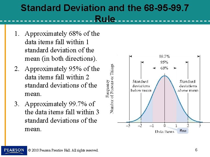
Standard Deviation and the 68 -95 -99. 7 Rule 1. Approximately 68% of the data items fall within 1 standard deviation of the mean (in both directions). 2. Approximately 95% of the data items fall within 2 standard deviations of the mean. 3. Approximately 99. 7% of the data items fall within 3 standard deviations of the mean. © 2010 Pearson Prentice Hall. All rights reserved. 6

Example 1: Finding Scores at a Specified Standard Deviation From the Mean Male adult heights in North America are approximately normally distributed with a mean of 70 inches and a standard deviation of 4 inches. Find the height that is 2 standard deviations above the mean. Solution: Height = mean + 2∙standard deviation = 70 + 2∙ 4 = 70 + 8 = 78 © 2010 Pearson Prentice Hall. All rights reserved. 7

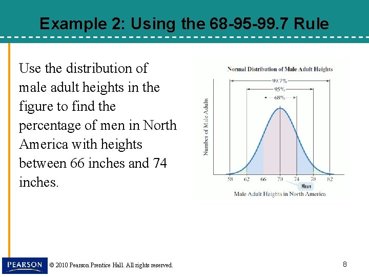
Example 2: Using the 68 -95 -99. 7 Rule Use the distribution of male adult heights in the figure to find the percentage of men in North America with heights between 66 inches and 74 inches. © 2010 Pearson Prentice Hall. All rights reserved. 8

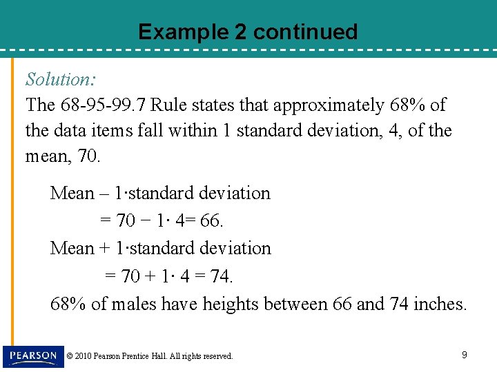
Example 2 continued Solution: The 68 -95 -99. 7 Rule states that approximately 68% of the data items fall within 1 standard deviation, 4, of the mean, 70. Mean – 1∙standard deviation = 70 − 1∙ 4= 66. Mean + 1∙standard deviation = 70 + 1∙ 4 = 74. 68% of males have heights between 66 and 74 inches. © 2010 Pearson Prentice Hall. All rights reserved. 9

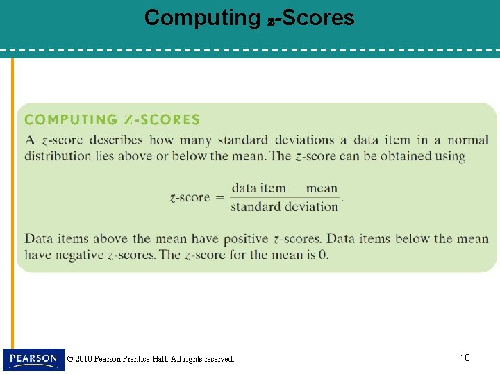
Computing z-Scores © 2010 Pearson Prentice Hall. All rights reserved. 10

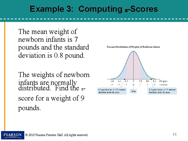
Example 3: Computing z-Scores The mean weight of newborn infants is 7 pounds and the standard deviation is 0. 8 pound. The weights of newborn infants are normally distributed. Find the zscore for a weight of 9 pounds. © 2010 Pearson Prentice Hall. All rights reserved. 11

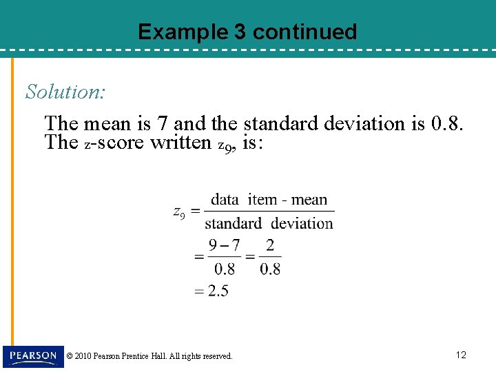
Example 3 continued Solution: The mean is 7 and the standard deviation is 0. 8. The z-score written z 9, is: © 2010 Pearson Prentice Hall. All rights reserved. 12

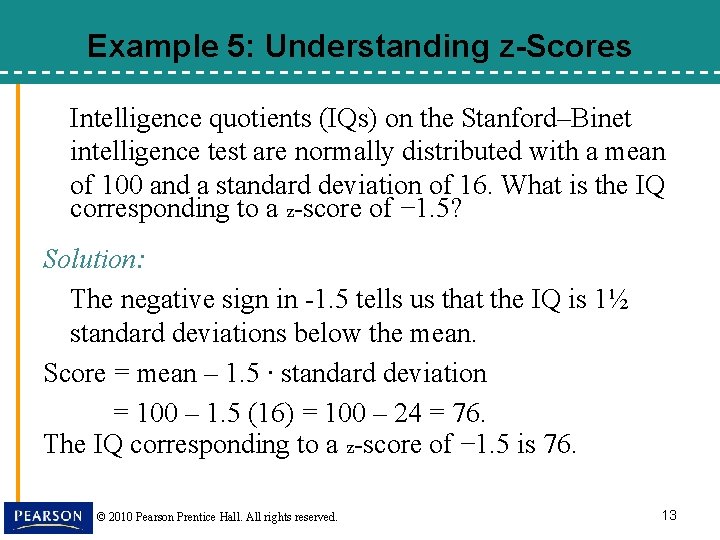
Example 5: Understanding z-Scores Intelligence quotients (IQs) on the Stanford–Binet intelligence test are normally distributed with a mean of 100 and a standard deviation of 16. What is the IQ corresponding to a z-score of − 1. 5? Solution: The negative sign in -1. 5 tells us that the IQ is 1½ standard deviations below the mean. Score = mean – 1. 5 ∙ standard deviation = 100 – 1. 5 (16) = 100 – 24 = 76. The IQ corresponding to a z-score of − 1. 5 is 76. © 2010 Pearson Prentice Hall. All rights reserved. 13

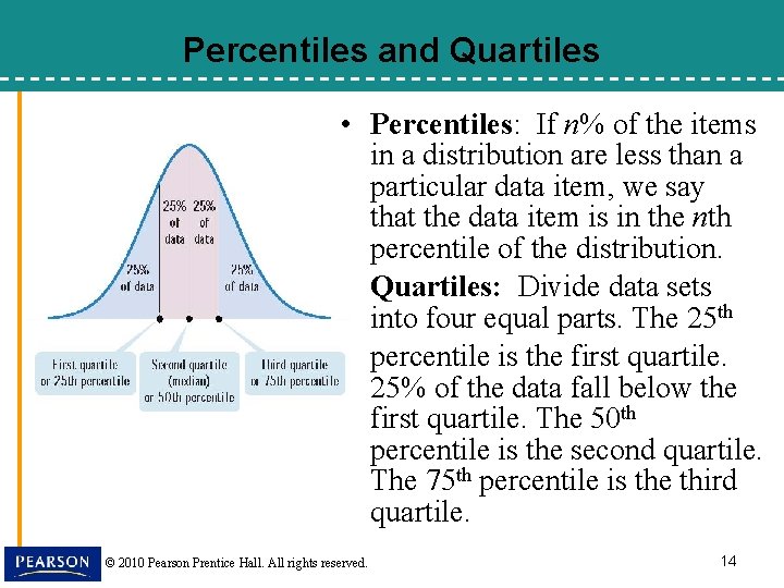
Percentiles and Quartiles • Percentiles: If n% of the items in a distribution are less than a particular data item, we say that the data item is in the nth percentile of the distribution. • Quartiles: Divide data sets into four equal parts. The 25 th percentile is the first quartile. 25% of the data fall below the first quartile. The 50 th percentile is the second quartile. The 75 th percentile is the third quartile. © 2010 Pearson Prentice Hall. All rights reserved. 14

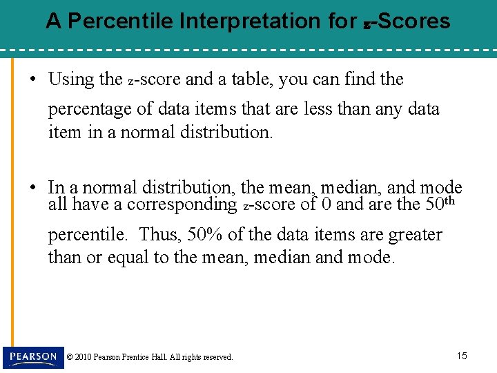
A Percentile Interpretation for z-Scores • Using the z-score and a table, you can find the percentage of data items that are less than any data item in a normal distribution. • In a normal distribution, the mean, median, and mode all have a corresponding z-score of 0 and are the 50 th percentile. Thus, 50% of the data items are greater than or equal to the mean, median and mode. © 2010 Pearson Prentice Hall. All rights reserved. 15

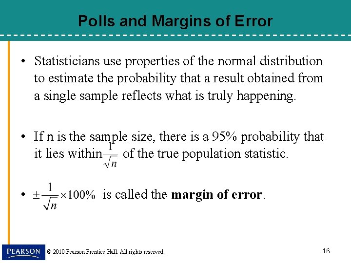
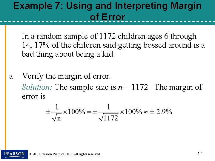
Polls and Margins of Error • Statisticians use properties of the normal distribution to estimate the probability that a result obtained from a single sample reflects what is truly happening. • If n is the sample size, there is a 95% probability that it lies within of the true population statistic. • is called the margin of error. © 2010 Pearson Prentice Hall. All rights reserved. 16

Example 7: Using and Interpreting Margin of Error In a random sample of 1172 children ages 6 through 14, 17% of the children said getting bossed around is a bad thing about being a kid. a. Verify the margin of error. Solution: The sample size is n = 1172. The margin of error is © 2010 Pearson Prentice Hall. All rights reserved. 17

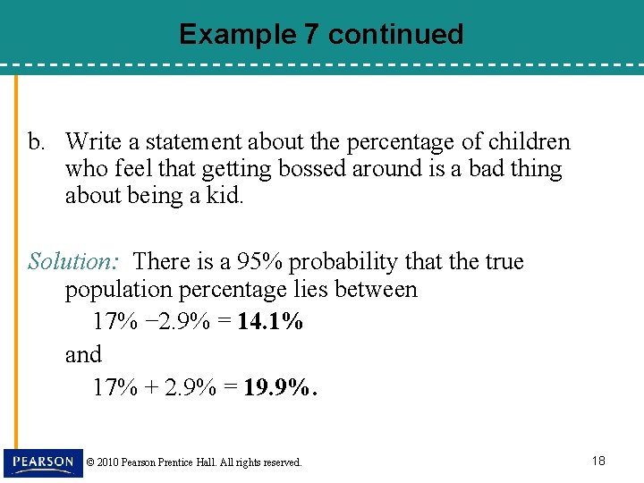
Example 7 continued b. Write a statement about the percentage of children who feel that getting bossed around is a bad thing about being a kid. Solution: There is a 95% probability that the true population percentage lies between 17% − 2. 9% = 14. 1% and 17% + 2. 9% = 19. 9%. © 2010 Pearson Prentice Hall. All rights reserved. 18

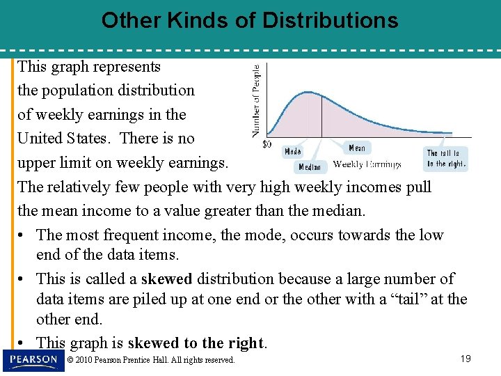
Other Kinds of Distributions This graph represents the population distribution of weekly earnings in the United States. There is no upper limit on weekly earnings. The relatively few people with very high weekly incomes pull the mean income to a value greater than the median. • The most frequent income, the mode, occurs towards the low end of the data items. • This is called a skewed distribution because a large number of data items are piled up at one end or the other with a “tail” at the other end. • This graph is skewed to the right. © 2010 Pearson Prentice Hall. All rights reserved. 19