Shareholders Required Rate of Return The Cost of

Shareholders’ Required Rate of Return (The Cost of Equity Capital) Chapter 6

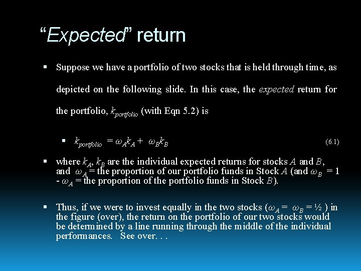
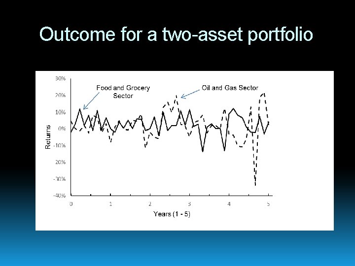
“Expected” return Suppose we have a portfolio of two stocks that is held through time, as depicted on the following slide. In this case, the expected return for the portfolio, kportfolio (with Eqn 5. 2) is kportfolio = ωAk. A + ωBk. B (6. 1) where k. A, k. B are the individual expected returns for stocks A and B, and ωA = the proportion of our portfolio funds in Stock A (and ωB = 1 - ωA = the proportion of the portfolio funds in Stock B). Thus, if we were to invest equally in the two stocks (ωA = ωB = ½ ) in the figure (over), the return on the portfolio of our two stocks would be determined by a line running through the middle of the individual performances. See over. . .

Outcome for a two-asset portfolio

Standard deviation of returns However, the variability of the returns of a portfolio comprising the two stocks is generally less than the weighted average of their variability individually. For example, if we observe the returns of the two stocks in the previous slide, we can see that the average return for the two stocks (a line running through the middle of the individual performances, but not depicted in the figure) is actually less “jerky” than for either of the two stocks individually. We may interpret this as the outcome of not putting all of one’s eggs in one basket. Or, we might say, the “swings and roundabouts” as the underperforming and over-performing price movements of the two stocks tend to cancel (at least somewhat) with each other.

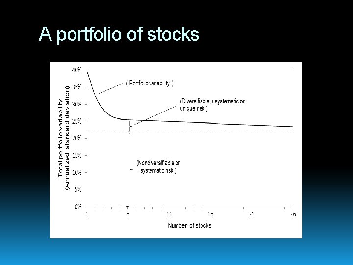
Standard deviation of returns (cont) We can therefore visualise that when we invest in many stocks – which of themselves are risky – we are actually less exposed to the risk of individual share performances than is the case when we invest only in a single stock. By investing in only one stock – putting all our eggs in one basket – we are very much at the mercy of a single company’s performance! However, with many stocks, the tendency of the stocks to either underperform or overperform against expectations will tend to cancel with one another - some of our stocks will pleasantly surprise us, while others will disappoint. We can imagine the relation as in the following figure, where with increasing number of stocks, the risk or variability of the portfolio’s returns is increasingly reduced. Next slide

A portfolio of stocks

A portfolio of stocks (cont) We note, however, that the risk or variability of the portfolio’s returns cannot be reduced to zero. This is due to the fact that all the stocks in the portfolio are connected to the market economy – so that when the market falters, all stocks are likely to be adversely affected by their exposure to the market. In this case, no matter how well we have “diversified” our portfolio, it cannot be completely protected against encountering a loss. Thus, in the figure, with increasing number of stocks, the risk or variability of portfolio returns continues to decrease – but only up to a point – from which, the portfolio’s market risk exposure remains. In other words, although the non-market (sometimes called nonsystematic or idiosyncratic) variability of stocks may be eliminated by holding a “well-diversified” portfolio, the market (sometimes called systematic or non-idiosyncratic) risk exposure of stocks due to their common dependence on the real economy cannot be eliminated by the expedient of diversification.

Market risk It is this market risk exposure – the risk that investors cannot diversify away by holding many shares - that demands a “market risk premium” (MRP) in the form of an expectation of return over and above a risk-free rate. Thus, we have the argument that the expected return on a stock should equal the risk-free rate plus the market risk premium in proportion to the stock’s beta – where beta is the measure of a stock’s sensitivity to the stock market. . This is the statement for the capital asset pricing model (CAPM), which was introduced in Chapter 1: k = r + β (MRP) j f j where kj is the required expectation of return for a Stock j; βj, the beta of firm j, measures the sensitivity or exposure of Stock j to the underlying economy; and MRP is the market “risk premium”.

The CAPM We may therefore express the CAPM as kj = rf + βj (MRP) = rf + βj [k. M - rf ] (6. 2) where we have represented the market risk premium (MRP) as the market’s expectation of return k. M over and above the rate rf offered by a risk-free asset (such as short-term government bonds) = k. M - rf. Thus, the CAPM as Eqn 6. 2 provides us with a model for shareholders’ required expectation of return as was applied in the discounting of dividends model of Chapter 5.

The CAPM (cont) In the CAPM as Eqn 6. 2, the risk-free rate (rf) and the market risk- premium (k. M - rf) are the same for all shares. Thus, on the right-hand side of the equation, it is only the beta that is related to the share in question. In effect, the CAPM represents a very bold statement, namely that different shares have different expectations of return that depend on their beta only. The security market line (SML) is a plot of the expectation of return (k) for an asset against the beta (β) of the asset.

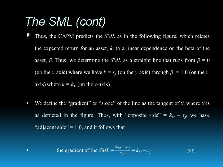
The SML (cont)

The SML

Inputs to the CAPM: the risk-free rate (rf) (i) The risk-free rate over a short-period may be taken as the rate on Treasury bills. But what for longer periods? As we observed in Chapter 4, the market’s anticipated interest rate is captured in the rate for longterm bonds. So a better approximation for the risk-free rate over a long period is likely to be the yield on a long-term government bond. But, as we also observed in Chapter 4, we encounter the problem that long-term government bonds are actually risky – not necessarily the risk that the government will dishonor the bond, but that the market value of the bonds – up or down - will fluctuate as inflation and interest rates fluctuate - down and up. The component of the yield on a long-term government Treasury bond that reflects a compensation for such risk exposure must therefore in principle be subtracted from the yield to reveal a longterm risk-free component. Thus, the risk-free rate is not entirely straightforward.

Inputs to the CAPM: the market risk premium (ii) Estimates for the market risk premium, as the market’s expectation of return over and above the risk-free rate, is also fraught with estimation problems. For example, prior to the global financial crisis, a stock market risk-premium in the range of 6– 8% was commonly referenced. Following the crisis, a more downbeat sentiment considered a market risk premium closer to 3. 5% as more realistically attainable, with estimates becoming more optimistic subsequently (with estimates closer to 6. 0%).

Inputs to the CAPM: beta (β) (iii) The beta (β) of the stock is the sensitivity of the stock to the market as the market goes through the economic cycle. If the stock’s return varies precisely as the market, its beta (β) = 1. If the stock’s return is more (less) sensitive to the market return – in other words, tending to exaggerate (suppress) the market’s performance – both on the market upturn and downturn – the stock beta is greater (less) than 1. 0. Sectors that might be expected to have a beta greater than 1 would be high -rise construction firms, purveyors of luxury items (top-of-the range cars, for example) and marketing firms, on account of that such items are likely to be curtailed in a recession. Sectors that might be expected to have a beta less than 1 would be such as retail supermarkets and alcohol, the former because we still need basic food items in the bad times, and the latter on account of that we tend to indulge in alcohol both to celebrate and to console ourselves.

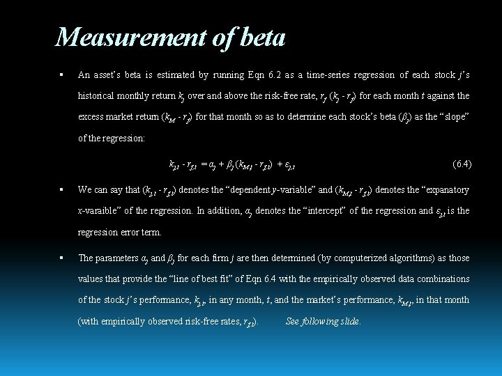
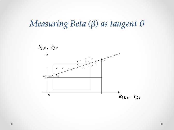
Measurement of beta An asset’s beta is estimated by running Eqn 6. 2 as a time-series regression of each stock j’s historical monthly return kj over and above the risk-free rate, rf (kj - rf) for each month t against the excess market return (k. M - rf) for that month so as to determine each stock’s beta (βj) as the “slope” of the regression: kj, t - rf, t = αj + βj (k. M, t - rf, t) + εj, t (6. 4) We can say that (kj, t - rf, t) denotes the “dependent y-variable” and (k. M, t - rf, t) denotes the “expanatory x-varaible” of the regression. In addition, αj denotes the “intercept” of the regression and εj, t is the regression error term. The parameters αj and βj for each firm j are then determined (by computerized algorithms) as those values that provide the “line of best fit” of Eqn 6. 4 with the empirically observed data combinations of the stock j’s performance, kj, t, in any month, t, and the market’s performance, k. M, t, in that month (with empirically observed risk-free rates, rf, t). See following slide.

Measuring Beta (β) as tangent θ

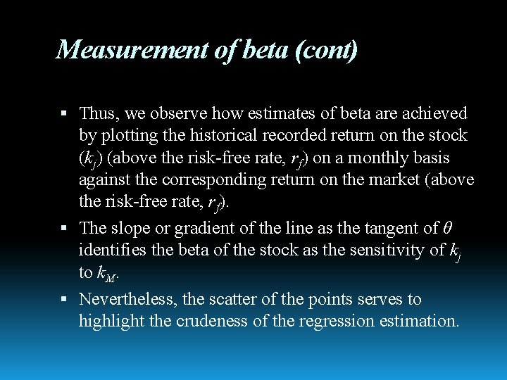
Measurement of beta (cont) Thus, we observe how estimates of beta are achieved by plotting the historical recorded return on the stock (kj) (above the risk-free rate, rf) on a monthly basis against the corresponding return on the market (above the risk-free rate, rf). The slope or gradient of the line as the tangent of θ identifies the beta of the stock as the sensitivity of kj to k. M. Nevertheless, the scatter of the points serves to highlight the crudeness of the regression estimation.

Break time

Empirical tests of the CAPM Logically, the risk premium for a particular asset should be in proportion to that asset’s sensitivity to the market. This is the statement of the CAPM. The statement appears to represent a perfectly acceptable principle of rational behavior, and following its introduction, a good deal of empirical work was performed aimed at supporting the prediction of the CAPM that an asset j’s expectation of return (kj) over the riskfree rate (rf) = kj – rf should be proportional to the asset’s exposure or sensitivity to the market, as measured by the asset’s beta (βj).

Testing the CAPM One response might be simply to ask anyone who holds stocks, either as individuals or as a portfolio or fund manager: What are your estimates of beta and expected return on each of the stocks you have chosen to hold? Then, test their responses against the model. Such an exercise would bring us to recognize that the concept of an investor’s expectation of return is actually quite a nebulous concept. Even sophisticated fund managers typically do not think explicitly in terms of expected returns on the stocks they hold, but, rather, of their portfolio of stocks in broad strategic terms, which is typically in accord with the mandate of the fund as entrusted to the fund trustees (that the fund invest in the firms of a given market index in proportion to each firm’s market value, for example).

Testing the CAPM (cont) In seeking to test the CAPM, the assumption is that each recorded monthly return for a stock is a random selection from the possible outcomes that were anticipated by investors on a probability-weighted basis for that stock at the outset of each month. We might imagine a sack with balls representing all possible outcomes in proportion to their probability of outcome (that is, outcome returns with a higher probability of outcome have proportionally more balls in the sack) and interpret each monthly return as a random selection from the sack.

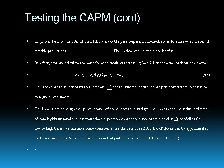
Testing the CAPM (cont) Empirical tests of the CAPM then follow a double-pass regression method, so as to achieve a number of testable predictions. In a first-pass, we calculate the betas for each stock by regressing Eqn 6. 4 on the data (as described above): The method can be explained briefly. kj, t - rf, t = αj + βj (k. M, t - rf, t) + εj, t (6. 4) The stocks are then ranked by their beta and 10 decile “bucket” portfolios are partitioned from lowest beta to highest beta stocks. The idea is that although the typical scatter of points about the straight line makes each individual estimate of beta highly uncertain, it is nevertheless expected that when the stocks are placed in 10 portfolios from low to high betas, we can have some confidence that the beta of each bucket of stocks can be approximated as the average beta (βP) beta of the stocks in that particular bucket portfolio (P = 1 → 10). /

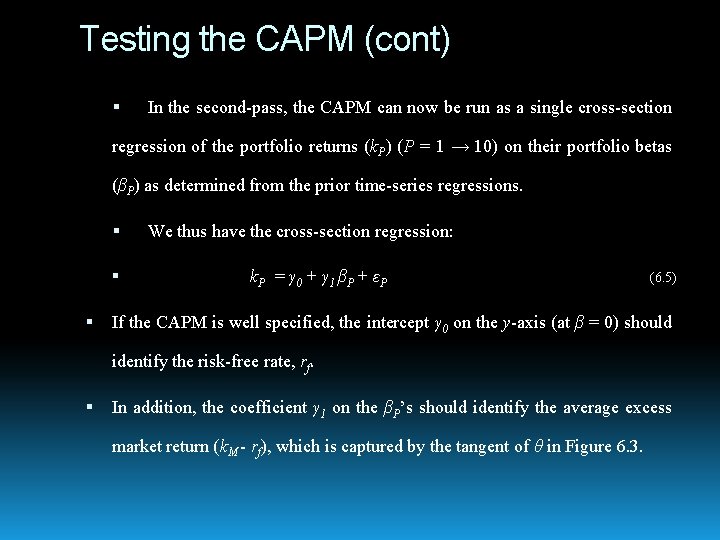
Testing the CAPM (cont) In the second-pass, the CAPM can now be run as a single cross-section regression of the portfolio returns (k. P) (P = 1 → 10) on their portfolio betas (βP) as determined from the prior time-series regressions. We thus have the cross-section regression: k P = γ 0 + γ 1 βP + εP (6. 5) If the CAPM is well specified, the intercept γ 0 on the y-axis (at β = 0) should identify the risk-free rate, rf. In addition, the coefficient γ 1 on the βP’s should identify the average excess market return (k. M - rf), which is captured by the tangent of θ in Figure 6. 3.

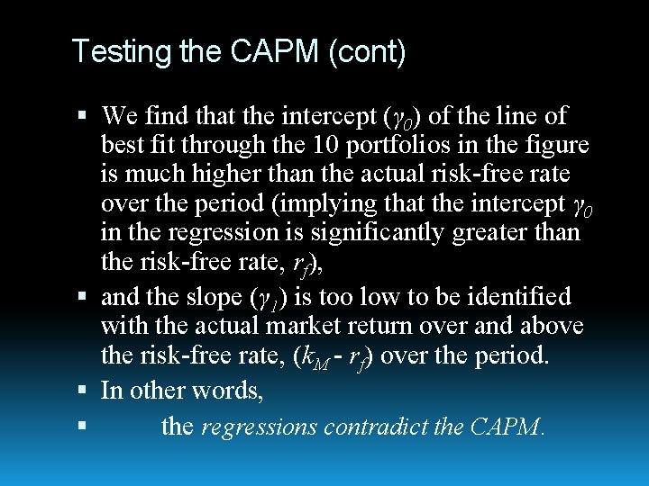
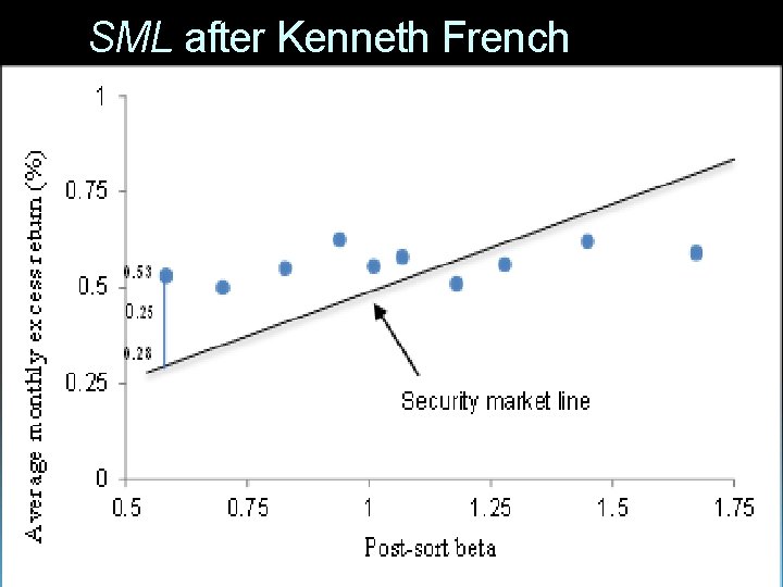
Testing the CAPM (cont) We find that the intercept (γ 0) of the line of best fit through the 10 portfolios in the figure is much higher than the actual risk-free rate over the period (implying that the intercept γ 0 in the regression is significantly greater than the risk-free rate, rf), and the slope (γ 1) is too low to be identified with the actual market return over and above the risk-free rate, (k. M - rf) over the period. In other words, the regressions contradict the CAPM.

SML after Kenneth French

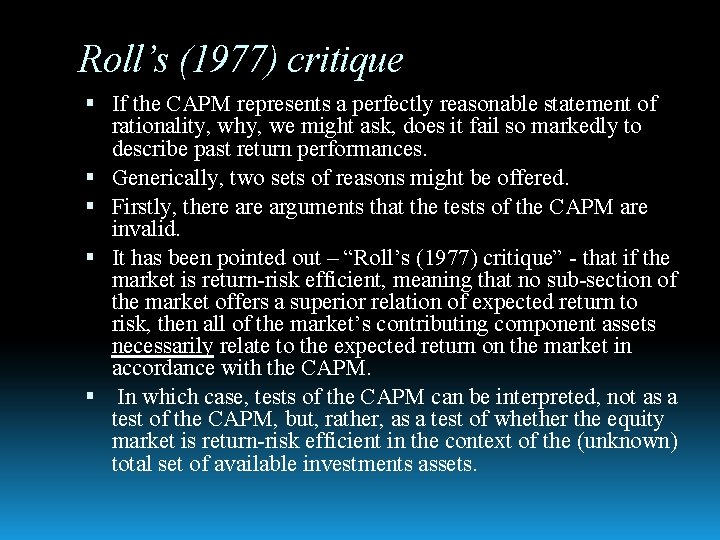
Roll’s (1977) critique If the CAPM represents a perfectly reasonable statement of rationality, why, we might ask, does it fail so markedly to describe past return performances. Generically, two sets of reasons might be offered. Firstly, there arguments that the tests of the CAPM are invalid. It has been pointed out – “Roll’s (1977) critique” - that if the market is return-risk efficient, meaning that no sub-section of the market offers a superior relation of expected return to risk, then all of the market’s contributing component assets necessarily relate to the expected return on the market in accordance with the CAPM. In which case, tests of the CAPM can be interpreted, not as a test of the CAPM, but, rather, as a test of whether the equity market is return-risk efficient in the context of the (unknown) total set of available investments assets.

The CAPM as irrelevant Secondly, it is possible that investors are sufficiently insensitive to beta as to actually disqualify the CAPM. In a world of disequilibrium, it may be that beta really is more or less irrelevant as institutional investors and professional portfolio managers compete in the business of picking winners in competition with other portfolio managers. A rational investor (investing h/h own money) might be aware of the commensurate downside to high beta stocks if the market should turn. But for institutional investors, as they compete for accolades of higher than average performance, the race is to the short run, over which they are assessed. For institutional investment, the risk is not the risk of losing (other people’s) money, but of underperforming against the competition.

The CAPM as irrelevant (cont) In Chapter 2, this was highlighted dramatically in the dot. com era and leading up to the GFC. Thus, when markets appear to be in the ascension, exposure to the market with higher beta stocks appears as a sensible strategy – with the longerterm downside potential of high beta stocks suppressed as a concern for risk. (“As long as the music is playing, you’ve got to get up and dance”. ) Justin Fox (2009) in The Myth of the Rational Market quotes a survey whereby professional investors, while agreeing pretty much unanimously that the Standard and Poor’s (S&P’s) price-to-earnings ratios in the high 20 s in 1999 would likely fall in the near future, nevertheless regarded that betting against such a drop could be a career killing move so long as the markets continued to grow. A case of the market can stay irrational longer than the rational institutional investor can keep his job. (“He was early, and there’s no difference between being early and being wrong”. ) In which case, an understanding of capital markets requires an understanding of the institutional imperatives encountered by fund managers rather than an understanding of individual stock sensitivities to beta.

The CAPM: Relevancy As an outcome of continued academic championing of the CAPM, the model has achieved broad acceptance in industry, as a model with which to estimate a firm’s cost of equity capital. And this is not necessarily irrational. If the principle of the CAPM is accepted, the model represents the logical determination of a rational shareholder’s long-term expectation of return for the firm (and its investments). Our point is that (for whatever reasons) the CAPM fails abjectly as an explanation of the observed formation of stock returns. We might say that the CAPM fails as a “capital asset pricing model” of markets, but remains as a valid “cost of equity formula” for the firm.

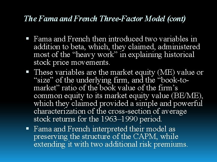
The Fama and French Three-Factor Model Altogether not actually the first to do so, in the early 1990 s, Eugene Fama and Kenneth French pronounced the ineffectiveness of the relation between historical average returns and beta (β). They observed, additionally, that the stocks of small firms tended to have both higher returns and higher betas, so that the higher returns for these firms could be attributed to the fact that the firms were small, rather than to their beta as such.

The Fama and French Three-Factor Model (cont) Fama and French then introduced two variables in addition to beta, which, they claimed, administered most of the “heavy work” in explaining historical stock price movements. These variables are the market equity (ME) value or “size” of the underlying firm, and the “book-tomarket” ratio of the book value of the firm’s common equity to its market equity value (BE/ME), which they claimed provided a simple and powerful characterization of the cross-section of average stock returns for the 1963– 1990 period. Fama and French interpreted their model as preserving the structure of the CAPM, while extending it with two additional risk premiums.

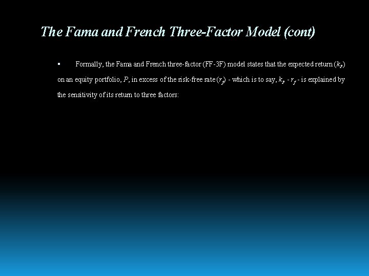
The Fama and French Three-Factor Model (cont) Formally, the Fama and French three-factor (FF-3 F) model states that the expected return (k. P) on an equity portfolio, P, in excess of the risk-free rate (rf) - which is to say, k. P - rf - is explained by the sensitivity of its return to three factors:

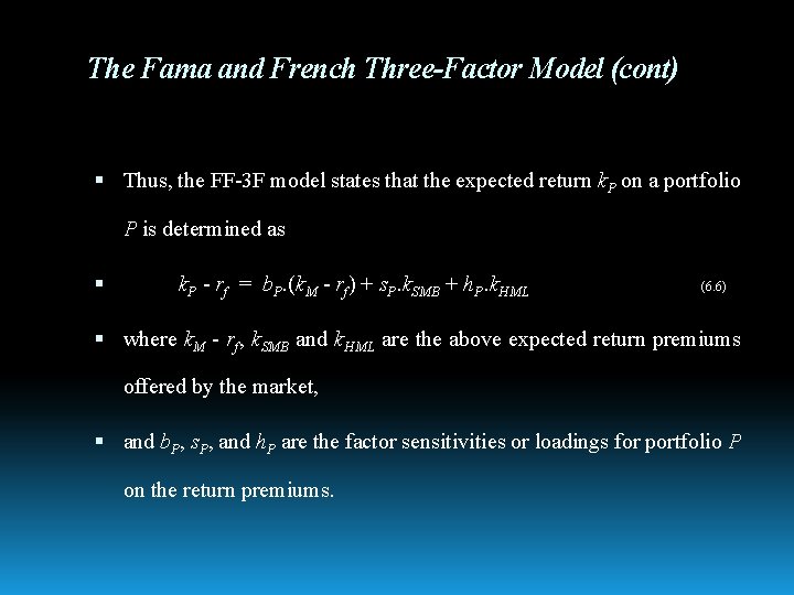
The Fama and French Three-Factor Model (cont) Thus, the FF-3 F model states that the expected return k. P on a portfolio P is determined as k. P - rf = b. P. (k. M - rf) + s. P. k. SMB + h. P. k. HML (6. 6) where k. M - rf, k. SMB and k. HML are the above expected return premiums offered by the market, and b. P, s. P, and h. P are the factor sensitivities or loadings for portfolio P on the return premiums.

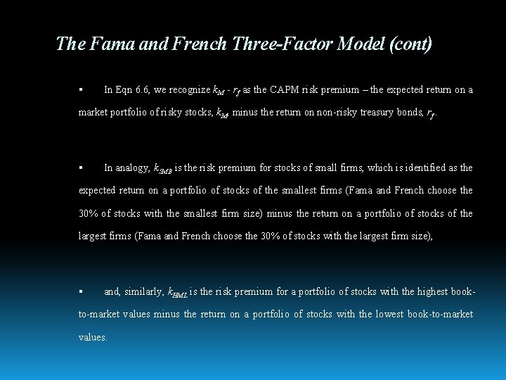
The Fama and French Three-Factor Model (cont) In Eqn 6. 6, we recognize k. M - rf as the CAPM risk premium – the expected return on a market portfolio of risky stocks, k. M, minus the return on non-risky treasury bonds, rf. In analogy, k. SMB is the risk premium for stocks of small firms, which is identified as the expected return on a portfolio of stocks of the smallest firms (Fama and French choose the 30% of stocks with the smallest firm size) minus the return on a portfolio of stocks of the largest firms (Fama and French choose the 30% of stocks with the largest firm size), and, similarly, k. HML is the risk premium for a portfolio of stocks with the highest book- to-market values minus the return on a portfolio of stocks with the lowest book-to-market values.

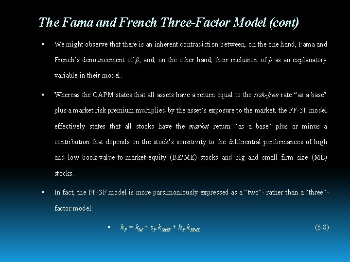
The Fama and French Three-Factor Model (cont) We might observe that there is an inherent contradiction between, on the one hand, Fama and French’s denouncement of β, and, on the other hand, their inclusion of β as an explanatory variable in their model. Whereas the CAPM states that all assets have a return equal to the risk-free rate “as a base” plus a market risk premium multiplied by the asset’s exposure to the market, the FF-3 F model effectively states that all stocks have the market return “as a base” plus or minus a contribution that depends on the stock’s sensitivity to the differential performances of high and low book-value-to-market-equity (BE/ME) stocks and big and small firm size (ME) stocks. In fact, the FF-3 F model is more parsimoniously expressed as a “two”- rather than a “three”factor model: k. P = k. M + s. P. k. SMB + h. P. k. HML (6. 8)

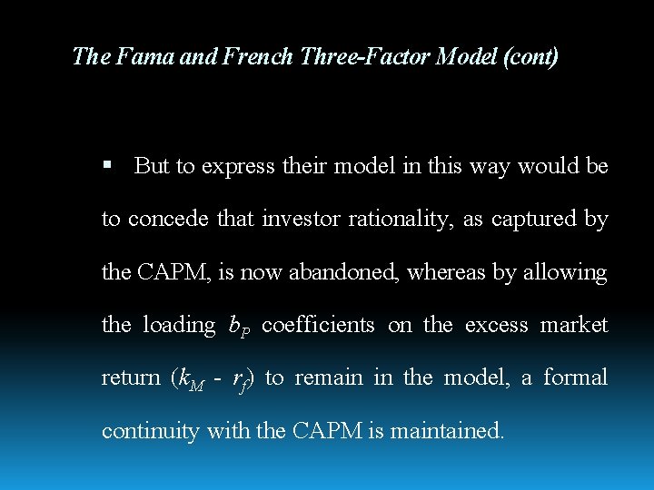
The Fama and French Three-Factor Model (cont) But to express their model in this way would be to concede that investor rationality, as captured by the CAPM, is now abandoned, whereas by allowing the loading b. P coefficients on the excess market return (k. M - rf) to remain in the model, a formal continuity with the CAPM is maintained.

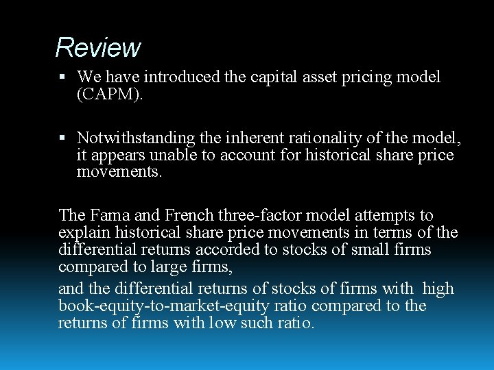
Review We have introduced the capital asset pricing model (CAPM). Notwithstanding the inherent rationality of the model, it appears unable to account for historical share price movements. The Fama and French three-factor model attempts to explain historical share price movements in terms of the differential returns accorded to stocks of small firms compared to large firms, and the differential returns of stocks of firms with high book-equity-to-market-equity ratio compared to the returns of firms with low such ratio.