Lecture 2 Price regulation Rate of Return Regulation

Lecture 2 Price regulation Rate of Return Regulation Tariff structure

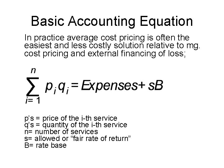
Basic Accounting Equation In practice average cost pricing is often the easiest and less costly solution relative to mg. cost pricing and external financing of loss; p’s = price of the i-th service q’s = quantity of the i-th service n= number of services s= allowed or “fair rate of return” B= rate base

Tasks of Regulator • Set allowed ‘normal’ profits, s and B; • Given profit levels, set prices to earn that profit; • Given one product this means average cost pricing; • For more than one product, there are sets of prices that satisfy equation (structure of prices); • Then Regulator needs to know demand elasticities

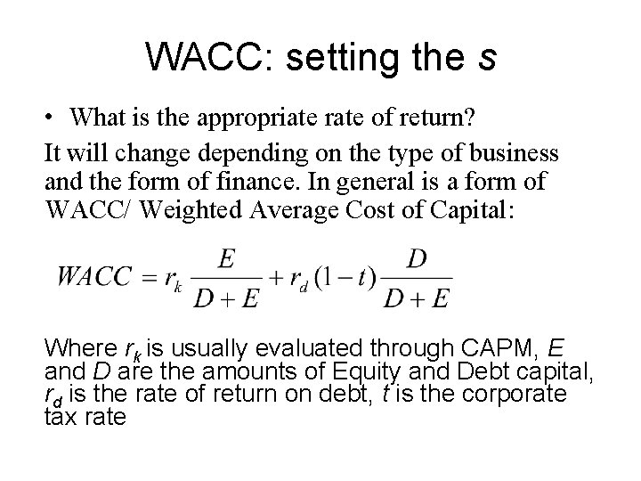
WACC: setting the s • What is the appropriate rate of return? It will change depending on the type of business and the form of finance. In general is a form of WACC/ Weighted Average Cost of Capital: Where rk is usually evaluated through CAPM, E and D are the amounts of Equity and Debt capital, rd is the rate of return on debt, t is the corporate tax rate

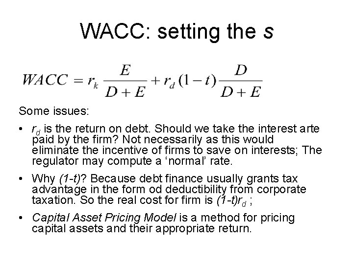
WACC: setting the s Some issues: • rd is the return on debt. Should we take the interest arte paid by the firm? Not necessarily as this would eliminate the incentive of firms to save on interests; The regulator may compute a ‘normal’ rate. • Why (1 -t)? Because debt finance usually grants tax advantage in the form od deductibility from corporate taxation. So the real cost for firm is (1 -t)rd ; • Capital Asset Pricing Model is a method for pricing capital assets and their appropriate return.

Regulatory Asset Base - In USA the most part of the regulatory review is devoted to discussion on approriate rate of return; in UK and Europe the focus is on Regulatory Asset Base (ES: dispute OFGAS-BG valuations differed by 65%); - Regulatory opportunism, the possibility that the regulator takes advantage of firms after they invested by not allowing some (capital) costs in the tariff calculation, may find an easy way of expression in the calculation of RAB;

Regulatory Asset Base The ‘used and useful’ doctrine: Capital expenditure is recognized in RAB for regulatory purposes only iff used and useful Why was it proposed? - Method to control the incentive to over-investment (Averch-Johnson); When any capital expenditure is recognized firms can invest more capital than useful; - But with demand uncertainty it may cause underinvestment - Under Price Cap is not very relevant

Valuation methods for Rate Base • Original cost; indexation • Reproduction cost: replacing capacity with old technology • Replacement costs: replacing capacity with newest technology • Value of outstanding stocks and bonds; circularity • Discounting of the revenue flow

Regulatory Asset Base Discounting of revenues: Circularity -Expected Revenues are de facto the regulated tariffs. So expectations determine the RAB which in turn determines the actual flow of revenues; -Need an anchor for the system; Must be based on some notion of efficient use of resources of society -Note that the problem of circularity is that any level of capital may be legitimated ex post; -Mistakes in RAB evaluation canot be corrected ex-post;

Regulatory Asset Base Indicative Value (water privat. in UK) uses the discounted revenue flow at ‘current regulatory practices’. That meant usually before privatization and reform;

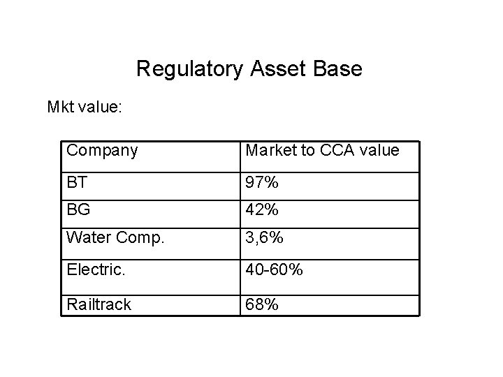
Regulatory Asset Base Market value (equity e debt): -The value of a firm is (broadly speaking) the discounted value of its revenue flow; -delegates to markets the task of forming expectations on regulated revenues; Circularity again is a problem; - Mistakes in the allowed rate of return are amplified by the discounting method (eg. low rate leads to low RAB) and lower overall remuneration; -May cause low RAB when there is regulatory risk; - Difficult to implement when the firm has both regulated and non-regulated business; - Nonetheless has been widely used at privatization in UK; -Good point: no windfall;

Regulatory Asset Base Mkt value: Company Market to CCA value BT 97% BG 42% Water Comp. 3, 6% Electric. 40 -60% Railtrack 68%

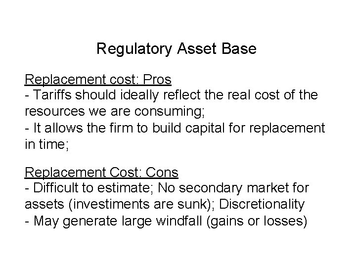
Regulatory Asset Base Replacement cost: Pros - Tariffs should ideally reflect the real cost of the resources we are consuming; - It allows the firm to build capital for replacement in time; Replacement Cost: Cons - Difficult to estimate; No secondary market for assets (investiments are sunk); Discretionality - May generate large windfall (gains or losses)

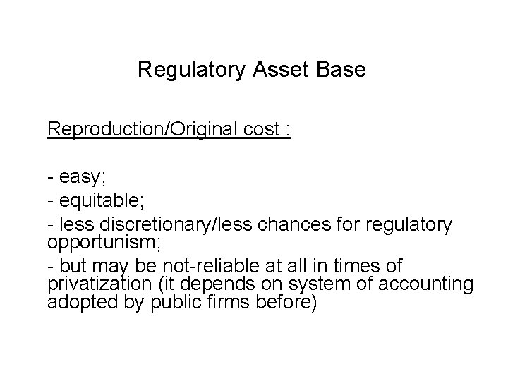
Regulatory Asset Base Reproduction/Original cost : - easy; - equitable; - less discretionary/less chances for regulatory opportunism; - but may be not-reliable at all in times of privatization (it depends on system of accounting adopted by public firms before)

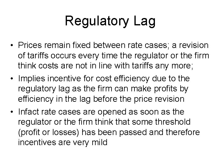
Regulatory Lag • Prices remain fixed between rate cases; a revision of tariffs occurs every time the regulator or the firm think costs are not in line with tariffs any more; • Implies incentive for cost efficiency due to the regulatory lag as the firm can make profits by efficiency in the lag before the price revision • Infact rate cases are opened as soon as the regulator or the firm think that some threshold (profit or losses) has been passed and therefore incentives are very mild

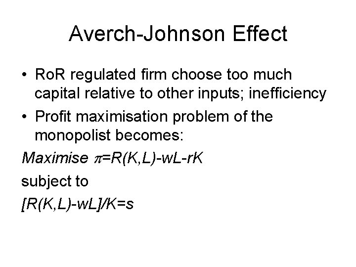
Averch-Johnson Effect • Ro. R regulated firm choose too much capital relative to other inputs; inefficiency • Profit maximisation problem of the monopolist becomes: Maximise =R(K, L)-w. L-r. K subject to [R(K, L)-w. L]/K=s

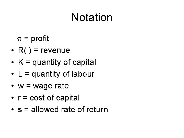
Notation • • • = profit R( ) = revenue K = quantity of capital L = quantity of labour w = wage rate r = cost of capital s = allowed rate of return

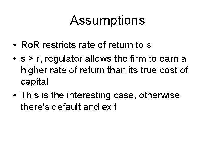
Assumptions • Ro. R restricts rate of return to s • s > r, regulator allows the firm to earn a higher rate of return than its true cost of capital • This is the interesting case, otherwise there’s default and exit

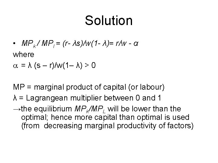
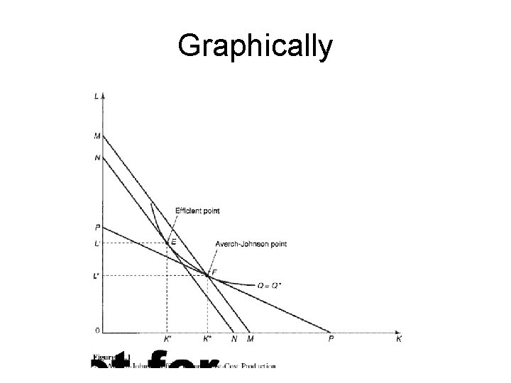
Solution • MPk / MPl = (r- λs)/w(1 - λ)= r/w - α where = λ (s – r)/w(1– λ) > 0 MP = marginal product of capital (or labour) λ = Lagrangean multiplier between 0 and 1 →the equilibrium MPk/MPL will be lower than the optimal; hence more capital than optimal is used (from decreasing marginal productivity of factors)

Graphically

Graphical Solution • Averch-Johnson point F: solution under rate-of -return regulation • E, Efficient, cost minimising point: solution of unregulated firm • Averch Johnson effect: Regulated firm uses more capital and less labour than optimal -bias towards capital • Excess costs measured in units of labour: distance on labour axis between iso-costline through efficient point and iso-costline through Averch-Johnson Point (MN)

Averch-Johnson Effect • Bias towards capital • excess costs measured in units of labour: distance on labour axis between isocostline through efficient point and isocostline through Averch Johnson Point • Capital intensive industries: stimulation of innovation, long distance phone calls • Retard innovations because of other effects

Incentive Regulation • The main problem of Ro. R is the lack of incentives to cost efficiency (and innovation) • Performance standards • Earnings share or sliding scale regulation encouraging cost reductions and efficiency enhancing strategies • Excess earnings are shared between the regulated firm and consumers. Year by year a fraction the excess profit is returned to consumers

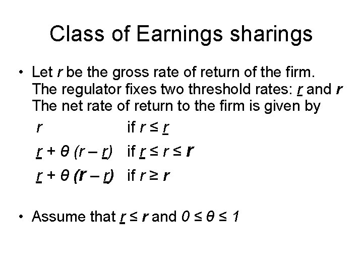
Class of Earnings sharings • Let r be the gross rate of return of the firm. The regulator fixes two threshold rates: r and r The net rate of return to the firm is given by r if r ≤ r r + θ (r – r) if r ≥ r • Assume that r ≤ r and 0 ≤ θ ≤ 1

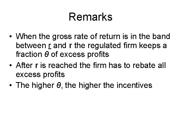
Remarks • When the gross rate of return is in the band between r and r the regulated firm keeps a fraction θ of excess profits • After r is reached the firm has to rebate all excess profits • The higher θ, the higher the incentives

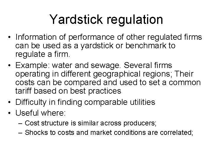
Yardstick regulation • Information of performance of other regulated firms can be used as a yardstick or benchmark to regulate a firm. • Example: water and sewage. Several firms operating in different geographical regions; Their costs can be compared and used to set a common tariff based on best practices • Difficulty in finding comparable utilities • Useful where: – Cost structure is similar across producers; – Shocks to costs and market conditions are correlated;

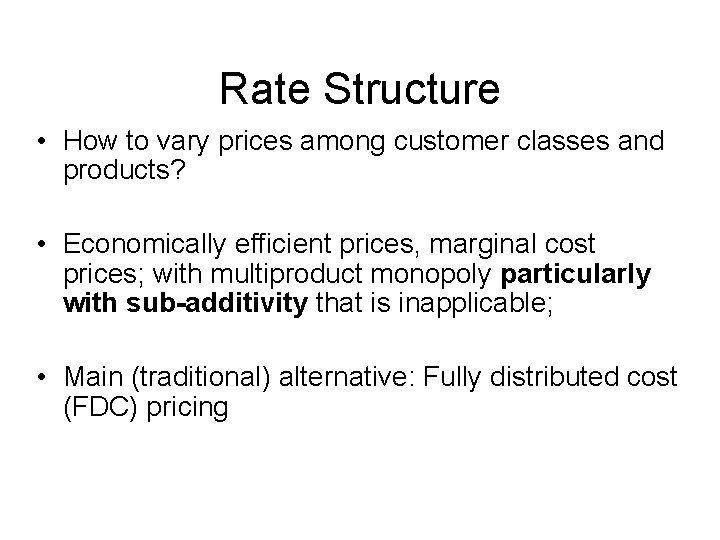
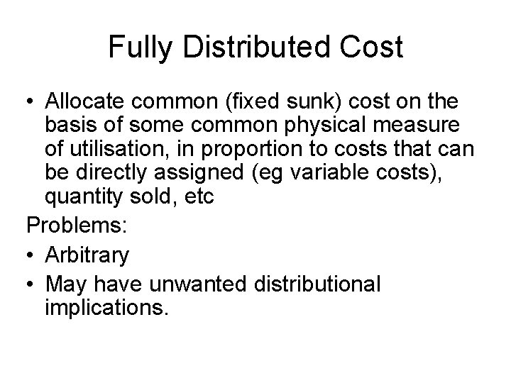
Rate Structure • How to vary prices among customer classes and products? • Economically efficient prices, marginal cost prices; with multiproduct monopoly particularly with sub-additivity that is inapplicable; • Main (traditional) alternative: Fully distributed cost (FDC) pricing

Fully Distributed Cost • Allocate common (fixed sunk) cost on the basis of some common physical measure of utilisation, in proportion to costs that can be directly assigned (eg variable costs), quantity sold, etc Problems: • Arbitrary • May have unwanted distributional implications.

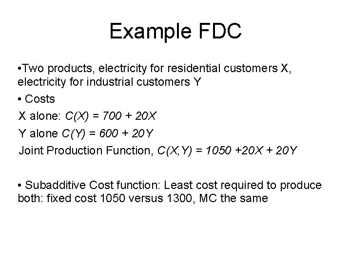
Example FDC • Two products, electricity for residential customers X, electricity for industrial customers Y • Costs X alone: C(X) = 700 + 20 X Y alone C(Y) = 600 + 20 Y Joint Production Function, C(X, Y) = 1050 +20 X + 20 Y • Subadditive Cost function: Least cost required to produce both: fixed cost 1050 versus 1300, MC the same

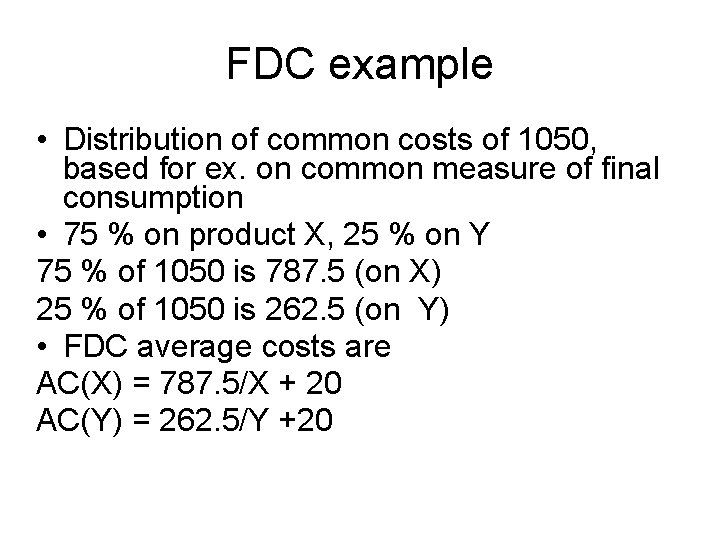
FDC example • Distribution of common costs of 1050, based for ex. on common measure of final consumption • 75 % on product X, 25 % on Y 75 % of 1050 is 787. 5 (on X) 25 % of 1050 is 262. 5 (on Y) • FDC average costs are AC(X) = 787. 5/X + 20 AC(Y) = 262. 5/Y +20

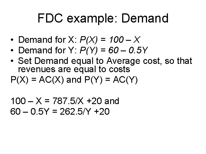
FDC example: Demand • Demand for X: P(X) = 100 – X • Demand for Y: P(Y) = 60 – 0. 5 Y • Set Demand equal to Average cost, so that revenues are equal to costs P(X) = AC(X) and P(Y) = AC(Y) 100 – X = 787. 5/X +20 and 60 – 0. 5 Y = 262. 5/Y +20

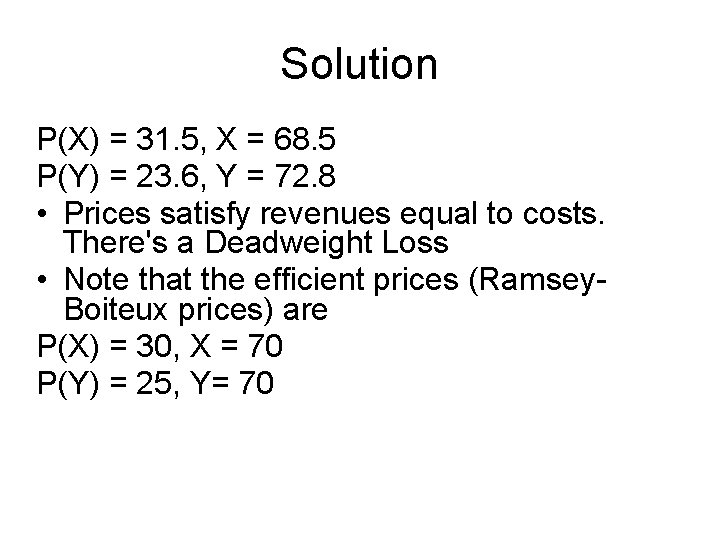
Solution P(X) = 31. 5, X = 68. 5 P(Y) = 23. 6, Y = 72. 8 • Prices satisfy revenues equal to costs. There's a Deadweight Loss • Note that the efficient prices (Ramsey. Boiteux prices) are P(X) = 30, X = 70 P(Y) = 25, Y= 70

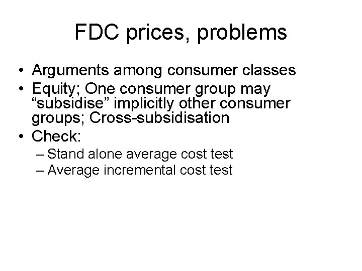
FDC prices, problems • Arguments among consumer classes • Equity; One consumer group may “subsidise” implicitly other consumer groups; Cross-subsidisation • Check: – Stand alone average cost test – Average incremental cost test

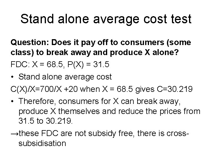
Stand alone average cost test Question: Does it pay off to consumers (some class) to break away and produce X alone? FDC: X = 68. 5, P(X) = 31. 5 • Stand alone average cost C(X)/X=700/X +20 when X = 68. 5 gives C=30. 219 • Therefore, consumers for X can break away, produce X themselves and reduce the prices from 31. 5 to 30. 219. →these FDC are not subsidy free, there is crosssubsidisation

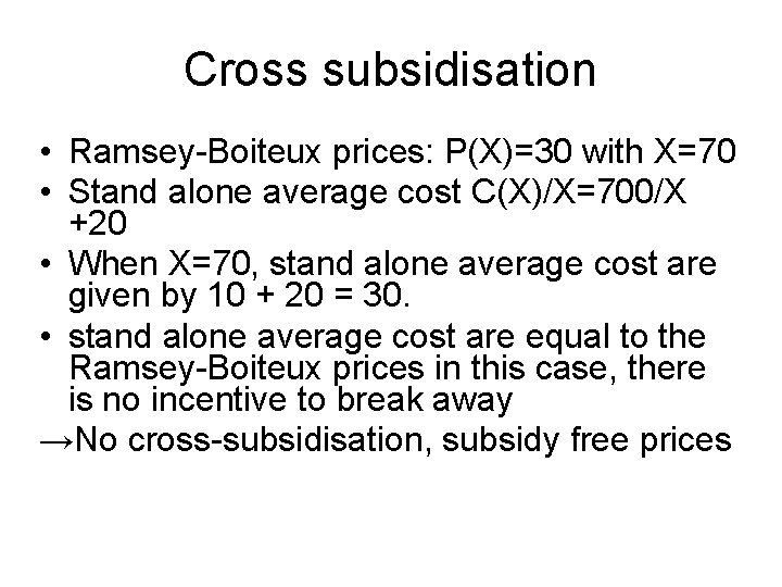
Cross subsidisation • Ramsey-Boiteux prices: P(X)=30 with X=70 • Stand alone average cost C(X)/X=700/X +20 • When X=70, stand alone average cost are given by 10 + 20 = 30. • stand alone average cost are equal to the Ramsey-Boiteux prices in this case, there is no incentive to break away →No cross-subsidisation, subsidy free prices

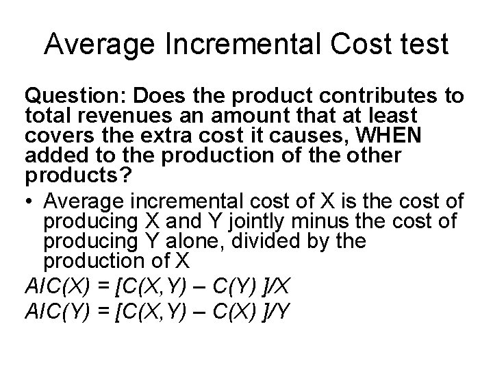
Average Incremental Cost test Question: Does the product contributes to total revenues an amount that at least covers the extra cost it causes, WHEN added to the production of the other products? • Average incremental cost of X is the cost of producing X and Y jointly minus the cost of producing Y alone, divided by the production of X AIC(X) = [C(X, Y) – C(Y) ]/X AIC(Y) = [C(X, Y) – C(X) ]/Y

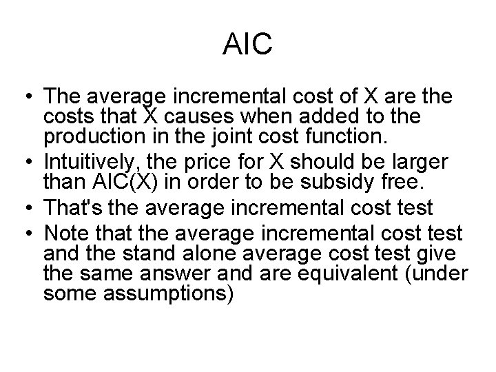
AIC • The average incremental cost of X are the costs that X causes when added to the production in the joint cost function. • Intuitively, the price for X should be larger than AIC(X) in order to be subsidy free. • That's the average incremental cost test • Note that the average incremental cost test and the stand alone average cost test give the same answer and are equivalent (under some assumptions)

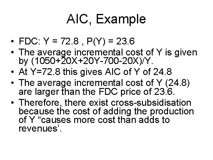
AIC, Example • FDC: Y = 72. 8 , P(Y) = 23. 6 • The average incremental cost of Y is given by (1050+20 X+20 Y-700 -20 X)/Y. • At Y=72. 8 this gives AIC of Y of 24. 8 • The average incremental cost of Y (24. 8) are larger than the FDC price of 23. 6. • Therefore, there exist cross-subsidisation because the cost of adding the production of Y “causes more cost than adds to revenues’.