Section 5 1 Review and Preview Review and

Section 5 -1 Review and Preview

Review and Preview This chapter combines the methods of descriptive statistics presented in Chapter 2 and 3 and those of probability presented in Chapter 4 to describe and analyze probability distributions. Probability Distributions describe what will probably happen instead of what actually did happen, and they are often given in the format of a graph, table, or formula.

Preview In order to fully understand probability distributions, we must first understand the concept of a random variable, and be able to distinguish between discrete and continuous random variables. In this chapter we focus on discrete probability distributions. In particular, we discuss binomial probability distributions.

Combining Descriptive Methods and Probabilities In this chapter we will construct probability distributions by presenting possible outcomes along with the relative frequencies we expect.

Section 5 -2 Random Variables

Random Variable Probability Distribution Random variable: a variable (typically represented by x) that has a single numerical value, determined by chance, for each outcome of a procedure. (Example: the number of peas with green pods among 5 offspring peas. ) Probability distribution: a description that gives the probability for each value of the random variable; often expressed in the format of a graph, table, or formula.

Discrete and Continuous Random Variables Discrete random variable: either a finite number of values or countable number of values, where “countable” refers to the fact that there might be infinitely many values, but they result from a counting process. (it cannot be a decimal) Continuous random variable: infinitely many values, and those values can be associated with measurements on a continuous scale without gaps or interruptions. (if something could be a decimal, it is continuous)

Example 1: Identify the given random variable as being discrete or continuous. a) The number of people now driving a car in the United States. Discrete b) The weight of the gold stored in Fort Knox. Continuous c) The height of the last airplane departed from JFK Airport in New York City. Continuous

Example 1 continued: Identify the given random variable as being discrete or continuous. d) The number of cars in San Francisco that crashed last year. Discrete e) The time required to fly from Los Angeles to Shanghai. Continuous

Requirements for Probability Distribution The sum of all probabilities is 1. ΣP(x) = 1, where x assumes all possible values. (Values such as 0. 999 or 1. 001 are acceptable due to roundoff error) Each individual probability is a value between 0 and 1 inclusive. 0 P(x) 1, for every individual value of x.

Mean, Variance and Standard Deviation of a Probability Distribution µ = Σ [x • P(x)] Mean 2 σ = Σ[(x – µ)2 • P(x)] 2 2 σ = Σ[x • P(x)] – µ σ= 2 Σ[x 2 • P(x)] – µ 2 Variance (shortcut) Standard Deviation

Roundoff Rule for µ, , and 2 Round results by carrying one more decimal place than the number of decimal places used for the random variable x. If the values of x are integers, round µ, σ, and σ2 to one decimal place.

Example 2: Determine whether or not a probability distribution is given. If a probability distribution is given, find its mean and standard deviation. If a probability distribution is not given, identify the requirement(s) that are not satisfied. Three males with X-linked genetic disorder have one child each. The random variable x is the number of children among the three who inherit the X-linked genetic disorder. x P(x) The given table is a probability distribution since 0 ≤ P(x) ≤ 1 for each x and ΣP(x) = 1. 0 0. 125 1 0. 375 2 0. 375 3 0. 125

Example 3: Determine whether or not a probability distribution is given. If a probability distribution is given, find its mean and standard deviation. If a probability distribution is not given, identify the requirement(s) that are not satisfied. Air America has a policy of routinely overbooking flights. The random variable x represents the number of passengers who cannot be boarded because there are more passengers than seats (based on data from an IBM research paper by Lawrence, Hong, and Cherrier. ) The given table is not a probability distribution since ΣP(x) = 0. 984 ≠ 1. x P(x) 0 0. 051 1 0. 141 2 0. 274 3 0. 331 4 0. 187

Example 4: Determine whether or not a probability distribution is given. If a probability distribution is given, find its mean and standard deviation. If a probability distribution is not given, identify the requirement(s) that is/are not satisfied. x P(x) The given table is not a probability distribution since ΣP(x) = 1. 2 ≠ 1. 1 0. 6 2 0. 2 3 0. 2 4 0. 15 5 0. 05

Identifying Unusual Results Range Rule of Thumb According to the range rule of thumb, most values should lie within 2 standard deviations of the mean. We can therefore identify “unusual” values by determining if they lie outside these limits: Maximum usual value = μ + 2σ Minimum usual value = μ – 2σ

Identifying Unusual Results Probabilities Rare Event Rule for Inferential Statistics If, under a given assumption (such as the assumption that a coin is fair), the probability of a particular observed event (such as 992 heads in 1000 tosses of a coin) is extremely small, we conclude that the assumption is probably not correct.

Identifying Unusual Results Probabilities Using Probabilities to Determine When Results Are Unusually high: x successes among n trials is an unusually high number of successes if P(x or more) ≤ 0. 05. Unusually low: x successes among n trials is an unusually low number of successes if P(x or fewer) ≤ 0. 05.

Example 5: Refer to the table, which describes results from eight offspring peas. The random variable x represents the number of offspring peas with green pods. a) Find the probability of getting exactly 7 peas with green pods. b) Find the probability of getting 7 or more peas with green pods. x P(x) 0 0+ 1 0+ 2 0. 004 3 0. 023 4 0. 087 5 0. 208 6 0. 311 7 0. 267 8 0. 100

Example 5 continued: Refer to the table, which describes results from eight offspring peas. The random variable x represents the number of offspring peas with green pods. x P(x) c) Which probability is relevant for determining whether 7 is an unusually high number of peas with green pods: the result from part (a) or part (b)? d) Is 7 an unusually high number of peas with green pods? Why or why not? 0 0+ 1 0+ 2 0. 004 3 0. 023 4 0. 087 5 0. 208 6 0. 311 7 0. 267 8 0. 100

Example 6: Based on past results found in the Information Please Almanac, there is a 0. 1919 probability that a baseball World Series contest will last four games, a 0. 2121 probability that it will last five games, a 0. 2222 probability that it will last six games, and a 0. 3737 probability that it will last seven games. a) Does the given information describe a probability distribution?

Example 6 continued: Based on past results found in the Information Please Almanac, there is a 0. 1919 probability that a baseball World Series contest will last four games, a 0. 2121 probability that it will last five games, a 0. 2222 probability that it will last six games, and a 0. 3737 probability that it will last seven games. b) Assuming that the given information describes a probability distribution, find the mean and standard deviation for the numbers of games in World Series contests.

Example 6 continued: Based on past results found in the Information Please Almanac, there is a 0. 1919 probability that a baseball World Series contest will last four games, a 0. 2121 probability that it will last five games, a 0. 2222 probability that it will last six games, and a 0. 3737 probability that it will last seven games. c) Is it unusual for a team to “sweep” by winning in four games? Why or why not?

Example 7: Based on data from Car. Max. com, when a car is randomly selected, the number of bumper stickers and the corresponding probabilities are as follows: 0 (0. 824); 1 (0. 083); 2 (0. 039); 3 (0. 014); 4 (0. 012); 5 (0. 008); 6 (0. 008); 7 (0. 004); 8 (0. 004); 9(0. 004). a) Does the given information describe a probability distribution?

Example 7 continued: Based on data from Car. Max. com, when a car is randomly selected, the number of bumper stickers and the corresponding probabilities are as follows: 0 (0. 824); 1 (0. 083); 2 (0. 039); 3 (0. 014); 4 (0. 012); 5 (0. 008); 6 (0. 008); 7 (0. 004); 8 (0. 004); 9(0. 004). b) Assuming that a probability distribution is described, find its mean and standard deviation.

Example 7 continued: Based on data from Car. Max. com, when a car is randomly selected, the number of bumper stickers and the corresponding probabilities are as follows: 0 (0. 824); 1 (0. 083); 2 (0. 039); 3 (0. 014); 4 (0. 012); 5 (0. 008); 6 (0. 008); 7 (0. 004); 8 (0. 004); 9(0. 004). c) Use the range rule of thumb to identify the range of values for usual numbers of bumper stickers.

Example 7 continued: Based on data from Car. Max. com, when a car is randomly selected, the number of bumper stickers and the corresponding probabilities are as follows: 0 (0. 824); 1 (0. 083); 2 (0. 039); 3 (0. 014); 4 (0. 012); 5 (0. 008); 6 (0. 008); 7 (0. 004); 8 (0. 004); 9(0. 004). d) Is it unusual for a car to have more than one bumper sticker? Why or why not?

Example 8: Let the random variable x represent the number of girls in a family of three children. Construct a table describing the probability distribution, then find the mean and standard deviation. (Hint: List the different possible outcomes) Is it unusual for a family of three children to consist of three girls?

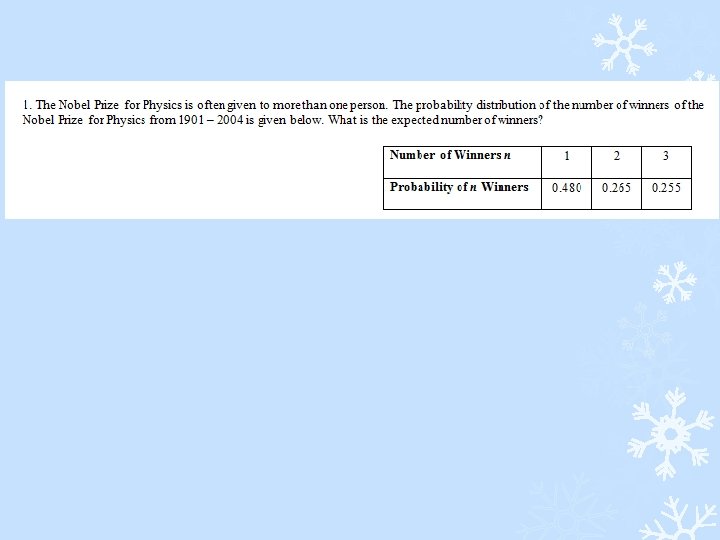
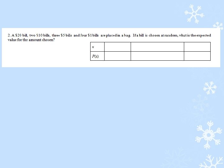
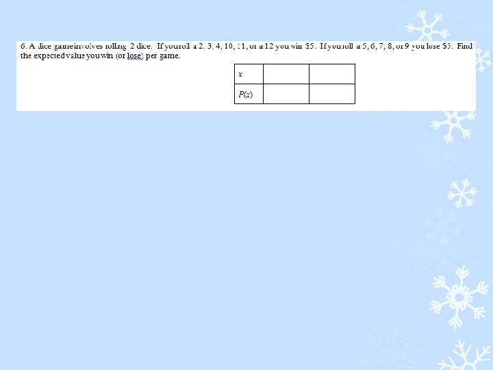
Expected Value The expected value of a discrete random variable is denoted by E, and it represents the mean value of the outcomes. It is obtained by finding the value of Σ [x • P(x)]. E = Σ[x • P(x)]

Example 9: In the Illinois Pick 3 lottery game, you pay 50¢ to select a sequence of three digits, such as 233. If you select the same sequence of three digits that are drawn, you win and collect $250. a) How many different selections are possible? b) What is the probability of winning? c) If you win, what is your net profit?

Example 9 continued: In the Illinois Pick 3 lottery game, you pay 50¢ to select a sequence of three digits, such as 233. If you select the same sequence of three digits that are drawn, you win and collect $250. d) Find the expected value. e) If you bet 50 ¢ in Illinois’ Pick 4 game, the expected value is – 25¢. Which bet is better: A 50¢ bet in the Illinois Pick 3 game or a 50¢ bet in the Illinois Pick 4 game? Explain.