Sampling plans for linear regression Given a domain

Sampling plans for linear regression • Given a domain, we can reduce the prediction error by good choice of the sampling points. • The choice of sampling locations is called “design of experiments” or DOE. • Will consider DOEs for linear regression using linear and quadratic polynomials and where errors are due to noise in the data. • With a given number of points the best DOE is one that will reduce the prediction variance (reviewed in next few slides). • The simplest DOE is full factorial design where we sample each variable (factor) at a fixed number of values (levels) • With k factors and three levels each we will sample 3 k points • Practical only for low dimensions • For vvuq course will cover slides 1, 5, 6, 9 -13, 14, 16

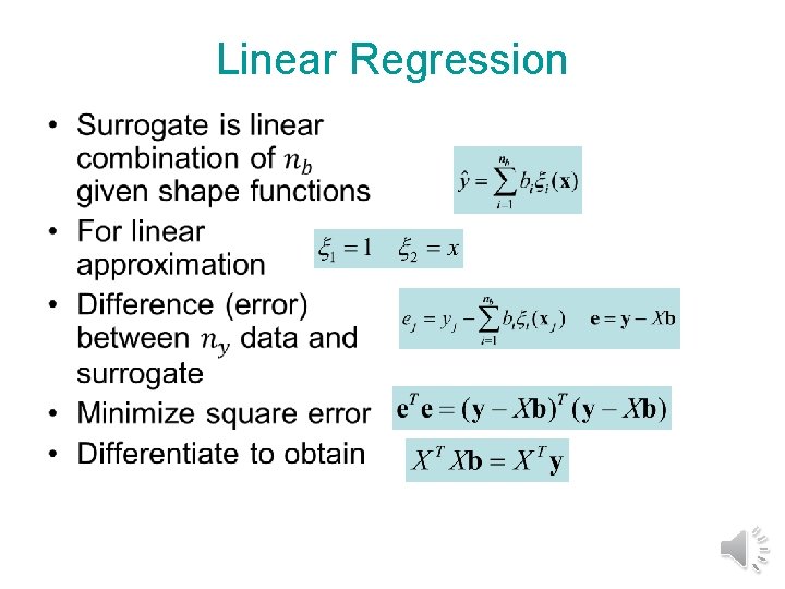
Linear Regression •

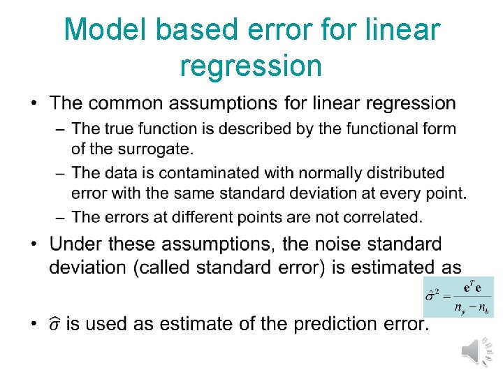
Model based error for linear regression •

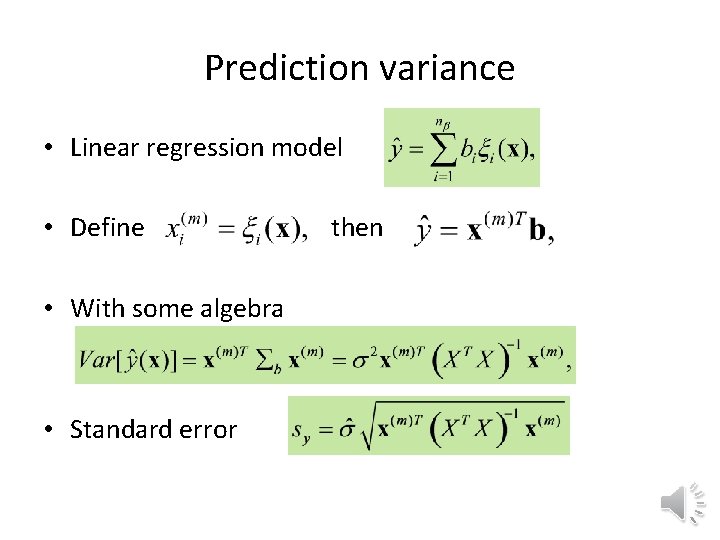
Prediction variance • Linear regression model • Define • With some algebra • Standard error then

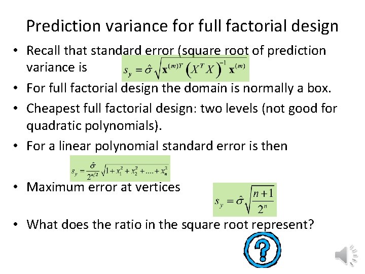
Prediction variance for full factorial design • Recall that standard error (square root of prediction variance is • For full factorial design the domain is normally a box. • Cheapest full factorial design: two levels (not good for quadratic polynomials). • For a linear polynomial standard error is then • Maximum error at vertices • What does the ratio in the square root represent?

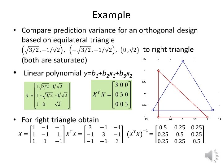
Designs for linear polynomials • Traditionally use only two levels. • Orthogonal design when XTX is diagonal. • Full factorial design is orthogonal, not so easy to produce other orthogonal designs with less points. • It is beneficial to place the points at the edges of the design domain. • Stability: Small variation of prediction variance in domain is also desirable property.

Example •

Comparison •

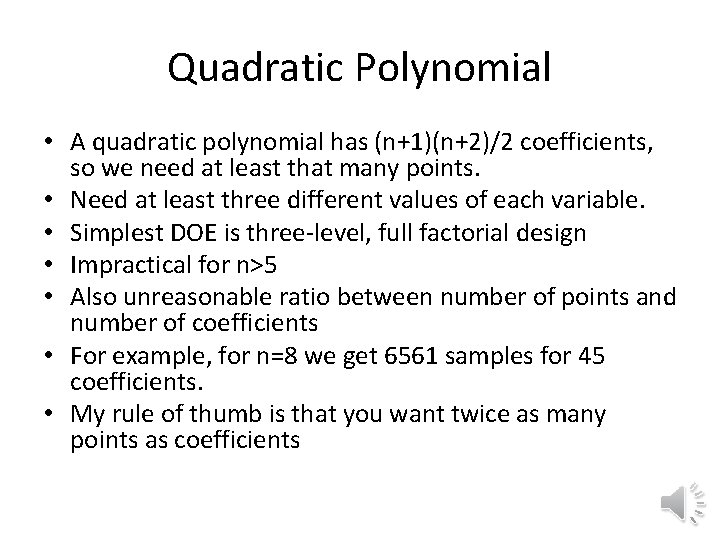
Quadratic Polynomial • A quadratic polynomial has (n+1)(n+2)/2 coefficients, so we need at least that many points. • Need at least three different values of each variable. • Simplest DOE is three-level, full factorial design • Impractical for n>5 • Also unreasonable ratio between number of points and number of coefficients • For example, for n=8 we get 6561 samples for 45 coefficients. • My rule of thumb is that you want twice as many points as coefficients

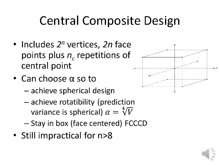
Central Composite Design •

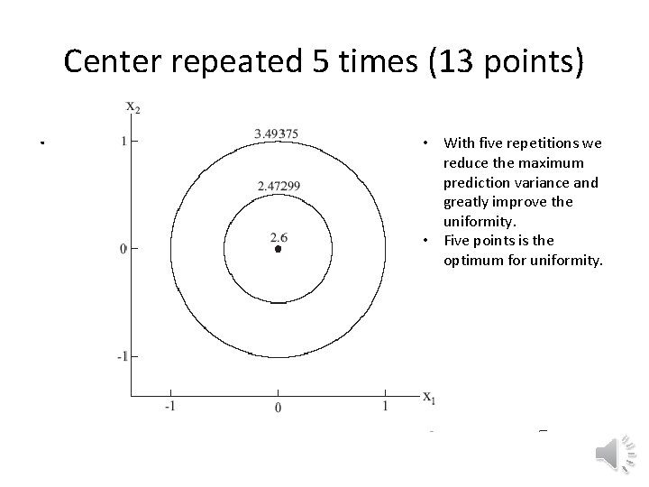
Repeated observations at origin • Unlike linear designs, prediction variance is high at origin. • Repetition at origin decreases variance there and improves stability. • What other rationale for choosing the origin for repetition? • Repetition also gives an independent measure of magnitude of noise. • Can be used also for lack-of-fit tests.

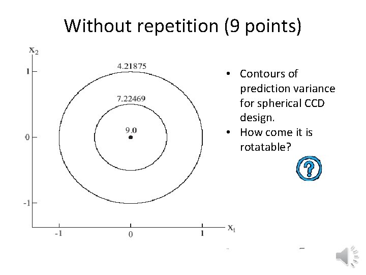
Without repetition (9 points) • Contours of prediction variance for spherical CCD design. • How come it is rotatable?

Center repeated 5 times (13 points). • With five repetitions we reduce the maximum prediction variance and greatly improve the uniformity. • Five points is the optimum for uniformity.

Top hat question • For the case of fitting a quadratic polynomial (6 coefficients) in two dimensions, we reduced the maximum prediction variance from 9 to 3. 5 by repeating the observation at the origin five times, requiring 13 observations instead of 9. • By what factor do you expect the prediction variance to change if you increased the number of points from 9 to 13 without targeting the point of highest variance? • 9/13; 3/7; 3/sqrt(13); sqrt(3/7)

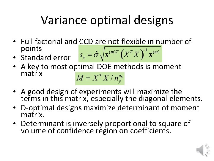
Variance optimal designs • Full factorial and CCD are not flexible in number of points • Standard error • A key to most optimal DOE methods is moment matrix • A good design of experiments will maximize the terms in this matrix, especially the diagonal elements. • D-optimal designs maximize determinant of moment matrix. • Determinant is inversely proportional to square of volume of confidence region on coefficients.

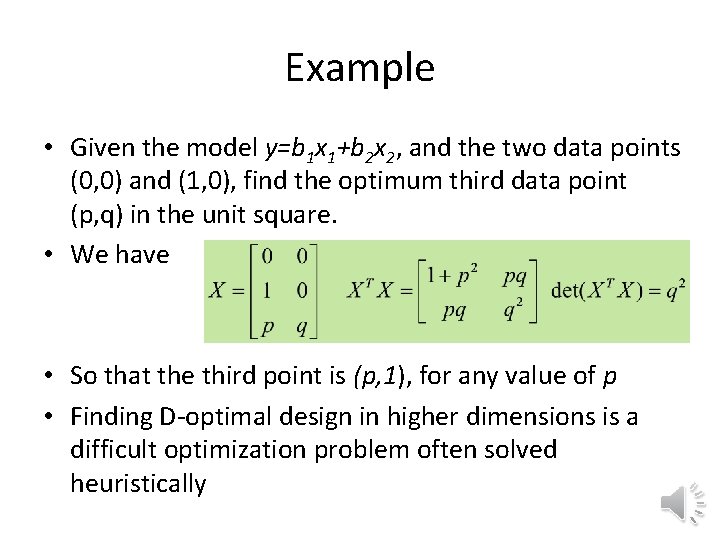
Example • Given the model y=b 1 x 1+b 2 x 2, and the two data points (0, 0) and (1, 0), find the optimum third data point (p, q) in the unit square. • We have • So that the third point is (p, 1), for any value of p • Finding D-optimal design in higher dimensions is a difficult optimization problem often solved heuristically

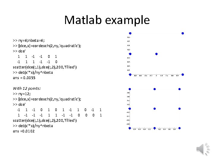
Matlab example >> ny=6; nbeta=6; >> [dce, x]=cordexch(2, ny, 'quadratic'); >> dce' 1 1 -1 0 1 -1 1 1 -1 0 scatter(dce(: , 1), dce(: , 2), 200, 'filled') >> det(x'*x)/ny^nbeta ans = 0. 0055 With 12 points: >> ny=12; >> [dce, x]=cordexch(2, ny, 'quadratic'); >> dce' -1 1 -1 0 1 -1 1 0 -1 1 1 -1 -1 0 0 0 1 scatter(dce(: , 1), dce(: , 2), 200, 'filled') >> det(x'*x)/ny^nbeta ans =0. 0102

Other criteria • A-optimal minimizes trace of the inverse of the moment matrix. • This minimizes the sum of the variances of the coefficients. • G-optimality minimizes the maximum of the prediction variance.

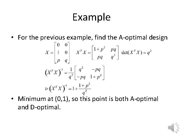
Example • For the previous example, find the A-optimal design • Minimum at (0, 1), so this point is both A-optimal and D-optimal.

Problems • Create a 13 -point D-optimal design in two dimensional space and compare its prediction variance to that of the CCD design shown on Slide 13. • Generate noisy data for the function y=(x+y)2 and fit using the two designs and compare the accuracy of the coefficients.