Richardson Extrapolation Romberg Integration and ODE Modifiers If

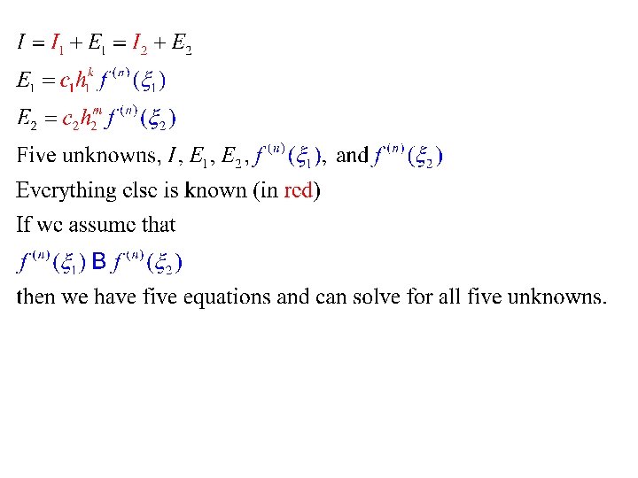
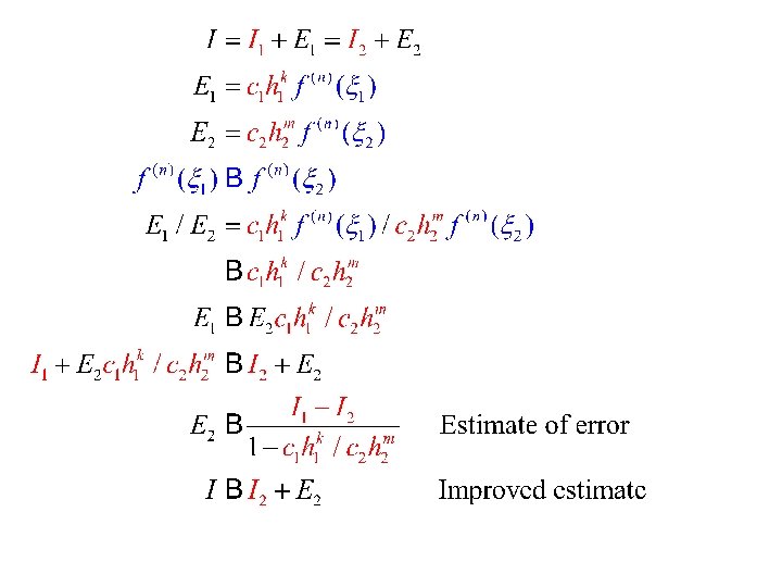
Richardson Extrapolation, Romberg Integration, and ODE Modifiers • If we have two estimates of the same thing, and error formulas, we can often make numerical estimates of the errors of the two methods • This can be used to improve the best estimate “for free” (no further function evaluations)

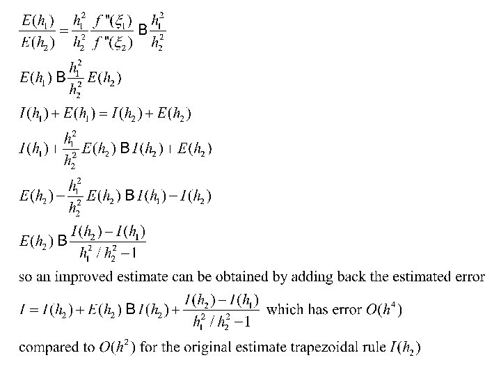
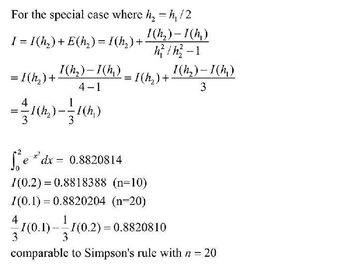
Repeated Richardson Extrapolation • With two separate O(h 2) estimates, we can combine them to make an O(h 4) estimate • With two separate O(h 4) estimates, we can combine them to make an O(h 6) estimate, etc. • The weights will be different for these repeated extrapolations

Errors for Richardson Extrapolation from Trapezoidal Rule Estimates n T 10 2 × 10 -4 R 1 R 2 4 × 10 -7 20 6 × 10 -5 5 × 10 -11 3 × 10 -8 40 2 × 10 -5

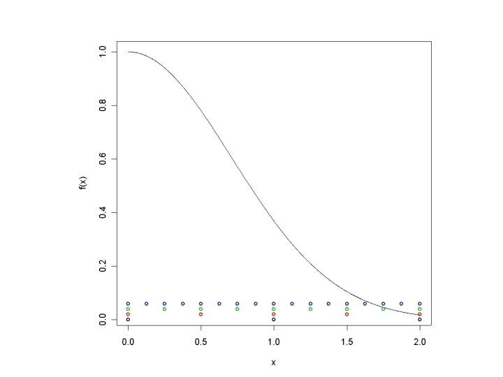
Romberg Integration • Romberg integration is an organized way of using Richardson extrapolation to obtain highly accurate estimates • Starts with the trapezoidal rule • Easily programmed

Romberg Integration • Let Ij, k represent an array of estimates of integrals • k = 1 represents trapezoid rules O(h 2) • k = 2 represents Richardson extrapolation from pairs of trapezoid rules O(h 4) • k = 3 represents Richardson extrapolation from pairs of the previous step at O(h 6), etc.

• If we double the number of points (halve the interval) at each step, then we only need to evaluate the function at the new points • For example, if the first step uses four intervals, it would involve evaluation at five points, the second one would use eight intervals, evaluated at nine points, only four of which are new

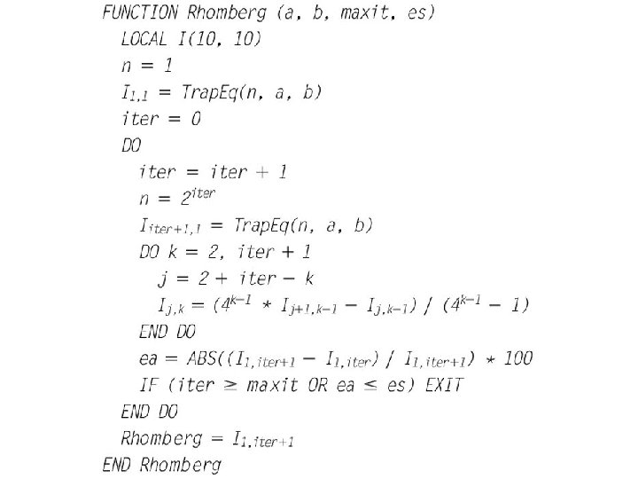
Design of Romberg Program • We start with the trapezoidal rule for one interval • We then add the trapezoidal rule for 2 intervals, plus the Richardson extrapolation • On each subsequent iteration, we add one more trapezoidal rule with twice the number of intervals • We then compute all the remaining possible Richardson extrapolations

Romberg starting with 2 intervals = 3 points 0. 8770373 0. 8818124 0. 8820814 0. 8806186 0. 8820655 0. 8820814 0. 0000000 0. 8817038 0. 8820804 0. 8820814 0. 0000000 0. 8819862 0. 8820813 0. 0000000 0. 8820576 0. 0000000 True value is 0. 8820814, requires 17 function evaluations to achieve 7 -digit accuracy. Simpson’s rule requires 36 function evaluations, and the trapezoid rule requires 775!

0. 8770373 0. 8818124 0. 8820814 0. 8806186 0. 8820655 0. 8820814 0. 0000000 0. 8817038 0. 8820804 0. 8820814 0. 0000000 0. 8819862 0. 8820813 0. 0000000 0. 8820576 0. 0000000

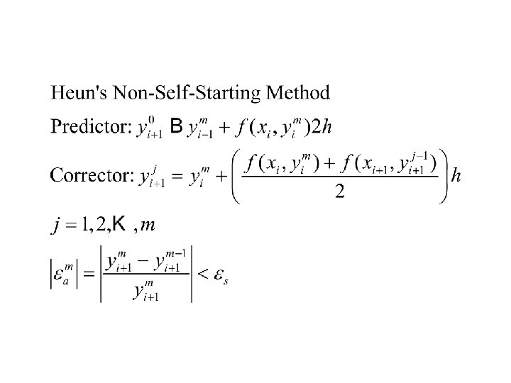
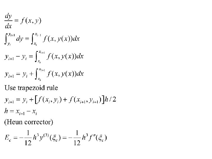
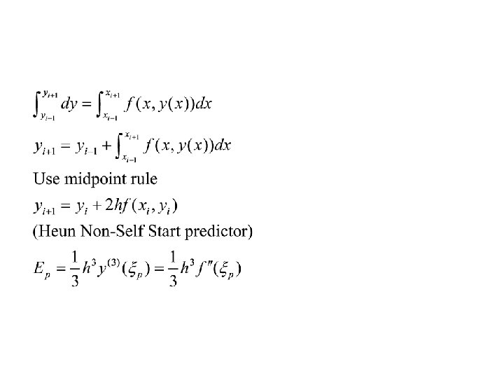
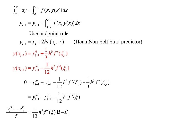
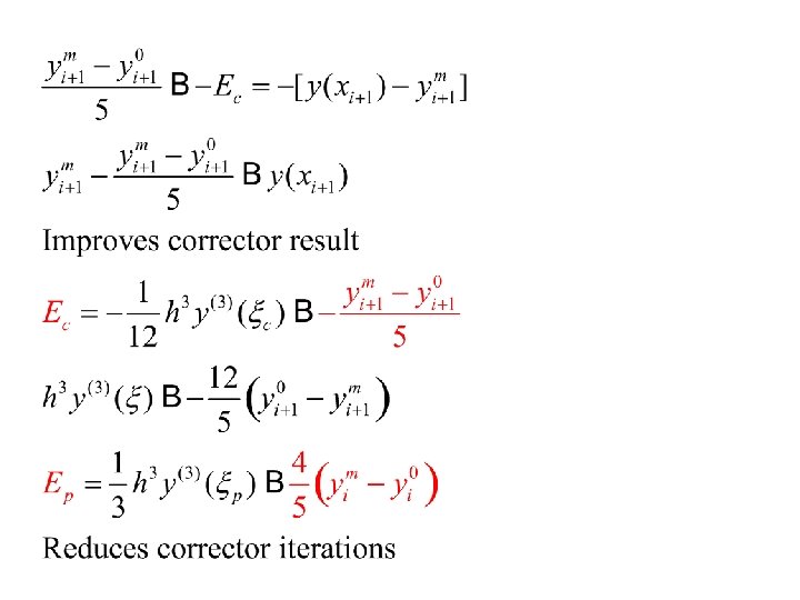
Heun’s Non-self-starting Method • This illustrates another use of the logic of estimating errors to improve the estimate • This is an example—we have seen many other such examples in the last lecture

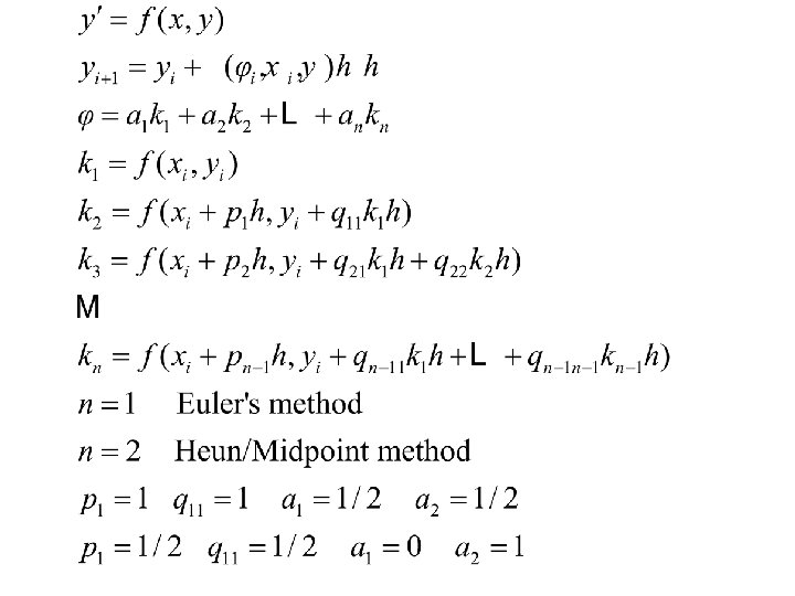
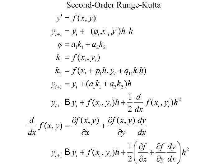
General Runge-Kutta Methods • Achieve accuracy of higher order Taylor series expansions without having to compute additional terms explicitly • Use the same general formulation as Euler’s method, Heun’s method, and the midpoint method in which the next point is the previous point plus the stepsize times an estimate of the slope.

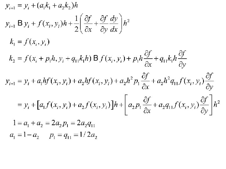
Determination of RK Coefficients • We pick the order of the method, which is the degree polynomial for which the method is exact, call this degree m. • We choose the coefficients of the RK method so as to integrate such polynomials exactly. More specifically, so that the order m Taylor approximation is integrated exactly.

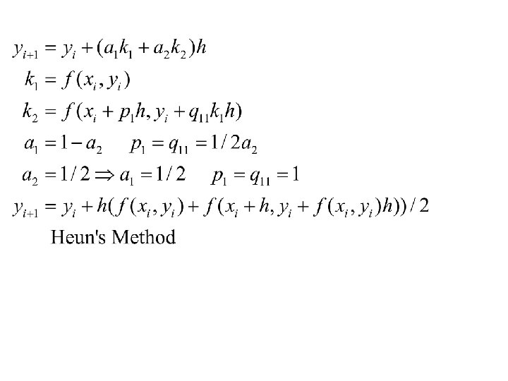
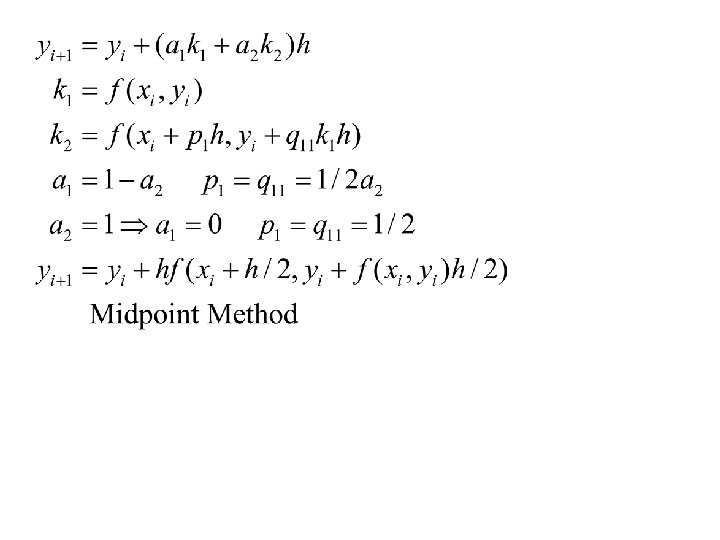
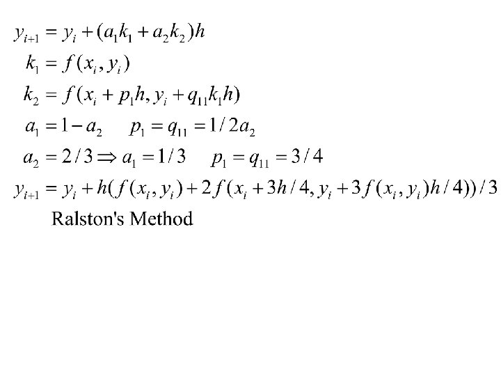
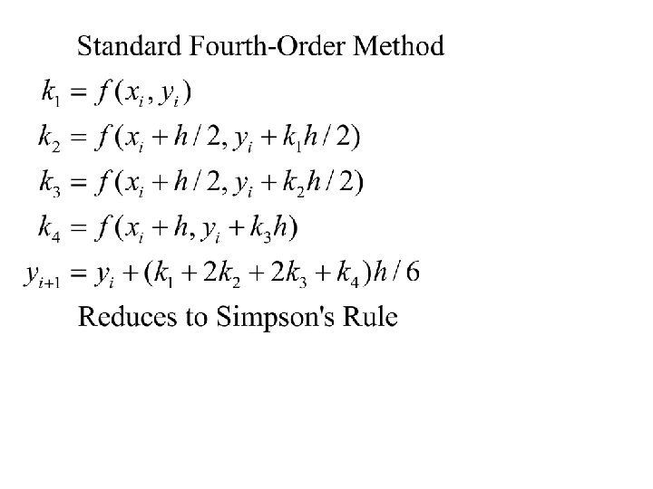
Higher-Order Methods • Euler’s method is RK order 1 and has global error O(h) • Second-order RK methods (Heun, Midpoint, Ralston) have global error O(h 2) • Third-order RK methods have global error O(h 3) • Fourth-order RK methods have global error O(h 4)

Derivation of RK Methods • Second-order RK methods have four constants, and three equations from comparing the Taylor series expansion to the iteration. There is one undetermined constant • Third-order methods have six equations with eight undetermined constants, so two are arbitrary.