PIOSSION STATISTICS Poisson process Poisson process is one

PIOSSION STATISTICS

Poisson process � Poisson process is one of the most important models used in queueing theory. � Often the arrival process of customers can be described by a Poisson process. � In teletra�c theory the “customers” may be calls or packets. Poisson process is a viable model when the calls or packets originate from a large population of independent users.

� Mathematically the process is described by the counter process Nt or N (t). The counter tells the number of arrivals that have occurred in the interval (0, t) or, more generally, in the interval (t 1, t 2) �N (t) = number of arrivals in the interval (0, t) � N (t 1 , t 2 ) = number of arrival in the interval (t 1 , t 2)

� The Poisson process can be defined in three di�erent (but equivalent) ways: � 1. Poisson process is a pure birth process: � In an infinite time interval dt there may occur λ only one arrival. This happens with the probability � λ dt independent of arrivals outside the interval.

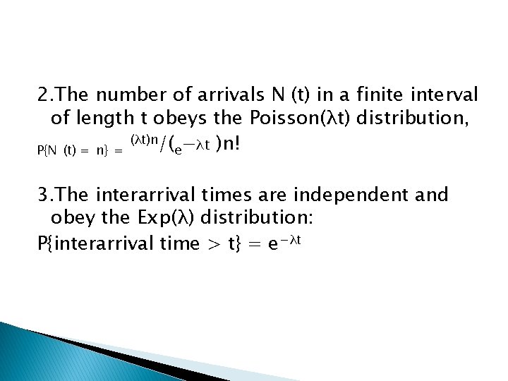
2. The number of arrivals N (t) in a finite interval of length t obeys the Poisson(λt) distribution, (λt)n/( −λt )n! P{N (t) = n} = e 3. The interarrival times are independent and obey the Exp(λ) distribution: P{interarrival time > t} = e−λt

History � The distribution was first introduced by Siméon Denis Poisson (1781– 1840) and published, together with his probability theory. � In 1837 in his work Research on the Probability of Judgments in Criminal and Civil Matters. � The work focused on certain random variables N that count, among other things, the number of discrete occurrences (sometimes called "events" or “arrivals”) that take place during a time-interval of given length.

� The Poisson distribution can also be used for the number of events in other specified intervals such as distance, area or volume. � For Example 4 pieces of mail per day on average. There will be, however, a certain spread: sometimes a little more, sometimes a little less, once in a while nothing at all. Given only the average rate, for a certain period of observation (pieces of mail per day, phonecalls per hour, etc. ), and assuming that the process, or mix of processes, that produces the event flow is essentially random, the Poisson distribution specifies how likely it is that the count will be 3, or 5, or 10, or any other number, during one period of observation. That is, it predicts the degree of spread around a known average rate of occurrence.

�A practical application of this distribution was made by Ladislaus Bortkiewicz in 1898 when he was given the task of investigating the number of soldiers in the russian army killed accidentally by horse kick; this experiment introduced the Poisson distribution to the field of reliability engineering.

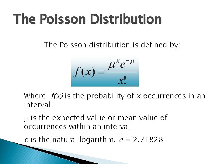
The Poisson Distribution The Poisson distribution is defined by: Where f(x) is the probability of x occurrences in an interval m is the expected value or mean value of occurrences within an interval e is the natural logarithm. e = 2. 71828

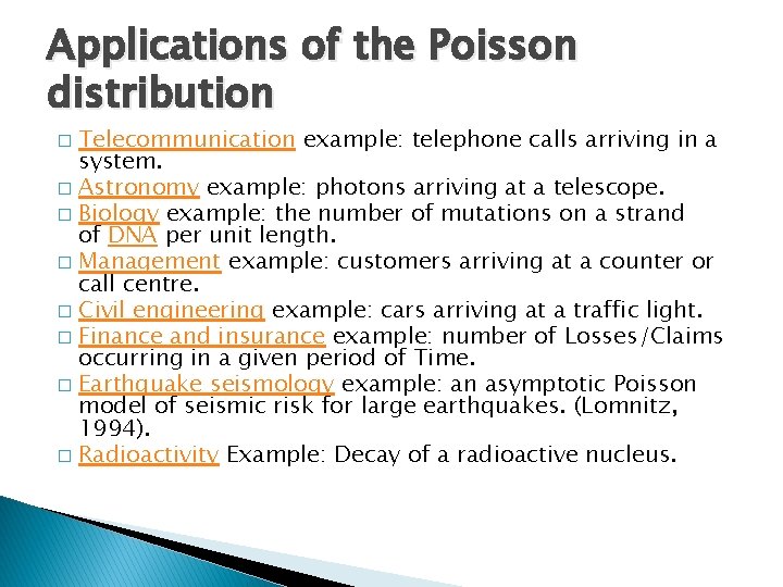
Applications of the Poisson distribution Telecommunication example: telephone calls arriving in a system. � Astronomy example: photons arriving at a telescope. � Biology example: the number of mutations on a strand of DNA per unit length. � Management example: customers arriving at a counter or call centre. � Civil engineering example: cars arriving at a traffic light. � Finance and insurance example: number of Losses/Claims occurring in a given period of Time. � Earthquake seismology example: an asymptotic Poisson model of seismic risk for large earthquakes. (Lomnitz, 1994). � Radioactivity Example: Decay of a radioactive nucleus. �

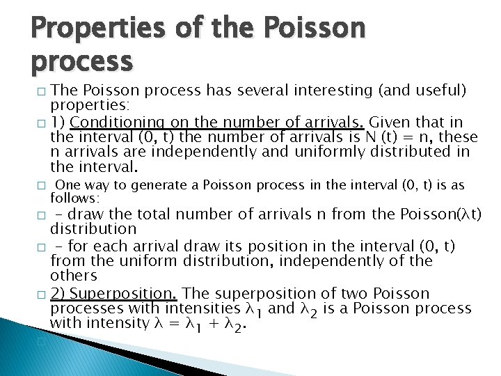
Properties of the Poisson process The Poisson process has several interesting (and useful) properties: � 1) Conditioning on the number of arrivals. Given that in the interval (0, t) the number of arrivals is N (t) = n, these n arrivals are independently and uniformly distributed in the interval. � � One way to generate a Poisson process in the interval (0, t) is as follows: – draw the total number of arrivals n from the Poisson(λt) distribution � – for each arrival draw its position in the interval (0, t) from the uniform distribution, independently of the others � 2) Superposition. The superposition of two Poisson processes with intensities λ 1 and λ 2 is a Poisson process with intensity λ = λ 1 + λ 2. � �

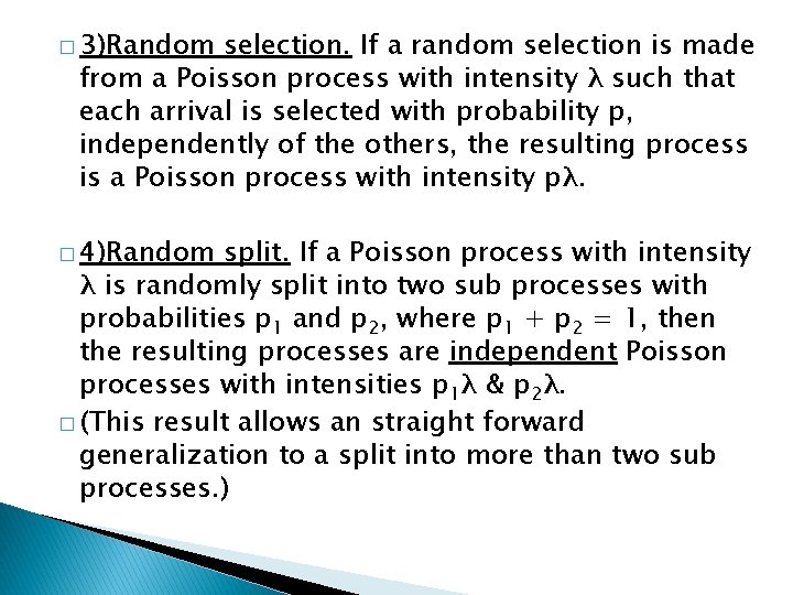
� 3)Random selection. If a random selection is made from a Poisson process with intensity λ such that each arrival is selected with probability p, independently of the others, the resulting process is a Poisson process with intensity pλ. � 4)Random split. If a Poisson process with intensity λ is randomly split into two sub processes with probabilities p 1 and p 2, where p 1 + p 2 = 1, then the resulting processes are independent Poisson processes with intensities p 1λ & p 2λ. � (This result allows an straight forward generalization to a split into more than two sub processes. )

� 5) PASTA. The Poisson process has the so called PASTA property (Poisson Arrivals See Time Averages): for instance, customers with Poisson arrivals see the system as if they came into the system at a random instant of time (despite they induce the evolution of the system).