Neural Networks Lecture 9 Learning in multilayer networks

Neural Networks Lecture 9: Learning in multi-layer networks Geoffrey Hinton

Preprocessing the input vectors • Instead of trying to predict the answer directly from the raw inputs we could start by extracting a layer of “features”. – Sensible if we already know that certain combinations of input values would be useful (e. g. edges or corners in an image). • Instead of learning the features we could design them by hand. – The hand-coded features are equivalent to a layer of non-linear neurons that do not need to be learned. – So far as the learning algorithm is concerned, the activities of the hand-coded features are the input vector.

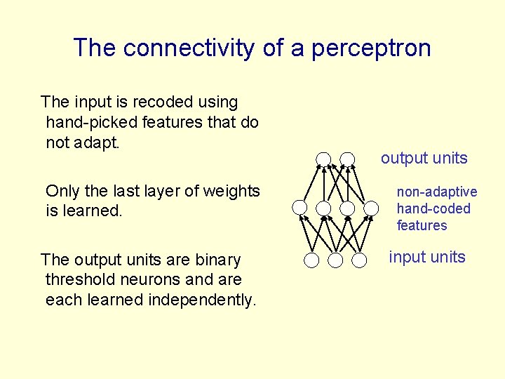
The connectivity of a perceptron The input is recoded using hand-picked features that do not adapt. Only the last layer of weights is learned. The output units are binary threshold neurons and are each learned independently. output units non-adaptive hand-coded features input units

Is preprocessing cheating? • It seems like cheating if the aim to show powerful learning is. The really hard bit is done by the preprocessing. • Its not cheating if we learn the non-linear preprocessing. – This makes learning much more difficult and much more interesting. . • Its not cheating if we use a very big set of nonlinear features that is task-independent. – Support Vector Machines make it possible to use a huge number of features without requiring much computation or data.

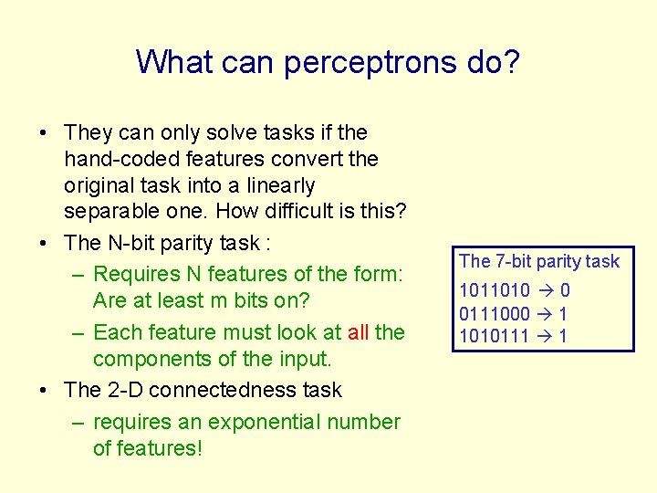
What can perceptrons do? • They can only solve tasks if the hand-coded features convert the original task into a linearly separable one. How difficult is this? • The N-bit parity task : – Requires N features of the form: Are at least m bits on? – Each feature must look at all the components of the input. • The 2 -D connectedness task – requires an exponential number of features! The 7 -bit parity task 1011010 0 0111000 1 1010111 1

Why connectedness is hard to compute • Even for simple line drawings, there are exponentially many cases. • Removing one segment can break connectedness – But this depends on the precise arrangement of the other pieces. – Unlike parity, there are no simple summaries of the other pieces that tell us what will happen. • Connectedness is easy to compute with an serial algorithm. – Start anywhere in the ink – Propagate a marker – See if all the ink gets marked.

Learning with hidden units • Networks without hidden units are very limited in the input-output mappings they can model. – More layers of linear units do not help. Its still linear. – Fixed output non-linearities are not enough • We need multiple layers of adaptive non-linear hidden units. This gives us a universal approximator. But how can we train such nets? – We need an efficient way of adapting all the weights, not just the last layer. This is hard. Learning the weights going into hidden units is equivalent to learning features. – Nobody is telling us directly what hidden units should do.

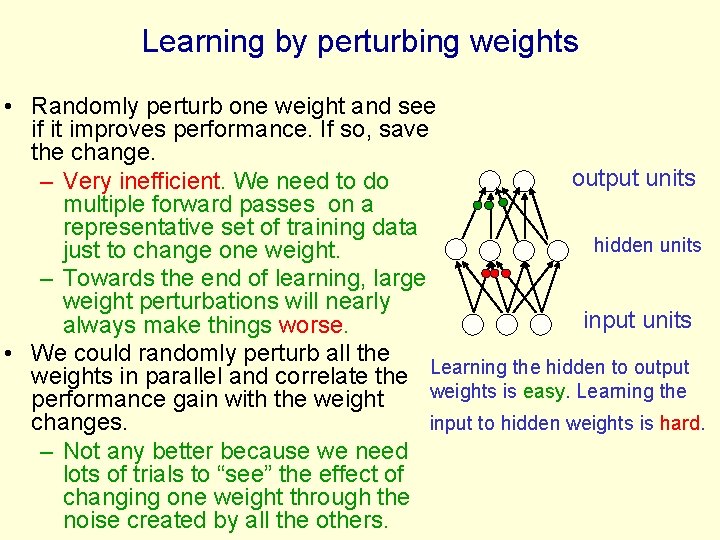
Learning by perturbing weights • Randomly perturb one weight and see if it improves performance. If so, save the change. output units – Very inefficient. We need to do multiple forward passes on a representative set of training data hidden units just to change one weight. – Towards the end of learning, large weight perturbations will nearly input units always make things worse. • We could randomly perturb all the weights in parallel and correlate the Learning the hidden to output weights is easy. Learning the performance gain with the weight input to hidden weights is hard. changes. – Not any better because we need lots of trials to “see” the effect of changing one weight through the noise created by all the others.

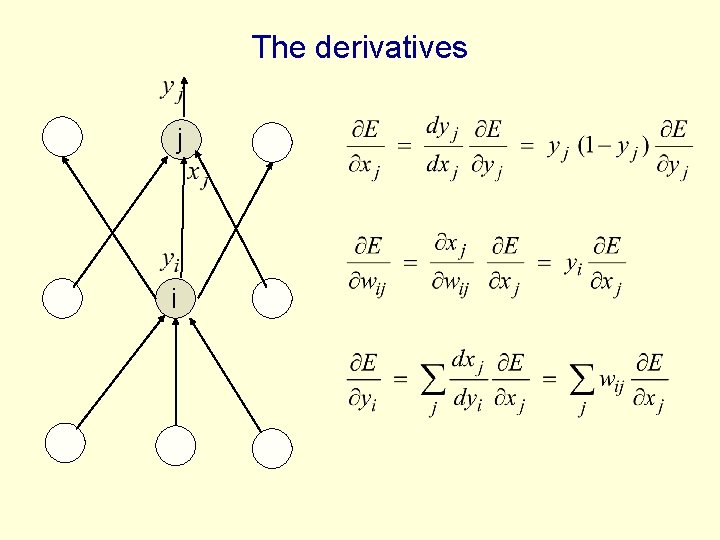
The idea behind backpropagation • We don’t know what the hidden units ought to do, but we can compute how fast the error changes as we change a hidden activity. – Instead of using desired activities to train the hidden units, use error derivatives w. r. t. hidden activities. – Each hidden activity can affect many output units and can therefore have many separate effects on the error. These effects must be combined. – We can compute error derivatives for all the hidden units efficiently. – Once we have the error derivatives for the hidden activities, its easy to get the error derivatives for the weights going into a hidden unit.

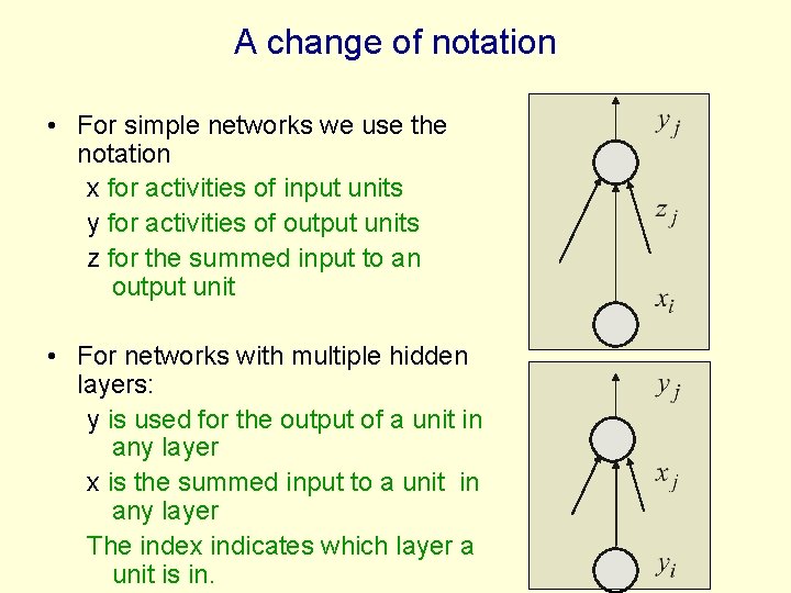
A change of notation • For simple networks we use the notation x for activities of input units y for activities of output units z for the summed input to an output unit • For networks with multiple hidden layers: y is used for the output of a unit in any layer x is the summed input to a unit in any layer The index indicates which layer a unit is in.

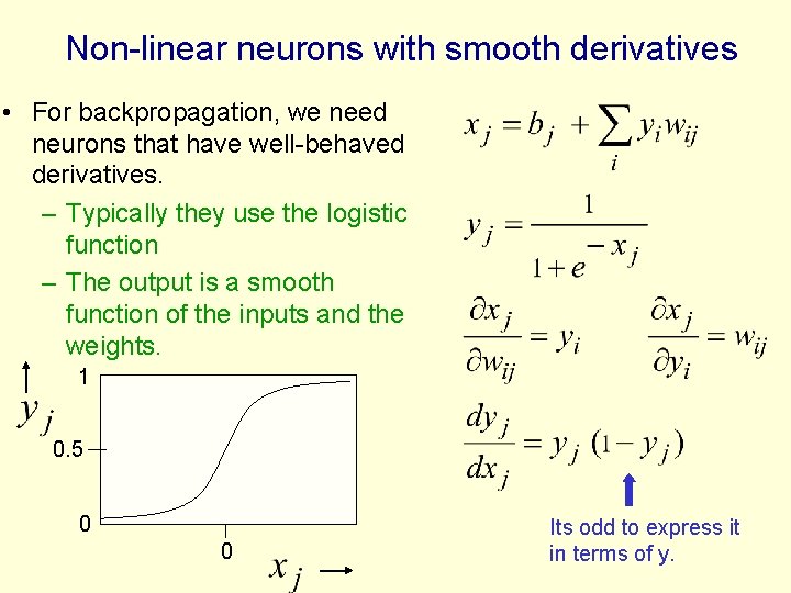
Non-linear neurons with smooth derivatives • For backpropagation, we need neurons that have well-behaved derivatives. – Typically they use the logistic function – The output is a smooth function of the inputs and the weights. 1 0. 5 0 0 Its odd to express it in terms of y.

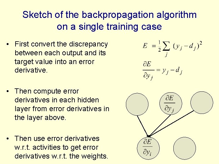
Sketch of the backpropagation algorithm on a single training case • First convert the discrepancy between each output and its target value into an error derivative. • Then compute error derivatives in each hidden layer from error derivatives in the layer above. • Then use error derivatives w. r. t. activities to get error derivatives w. r. t. the weights.

The derivatives j i

Ways to use weight derivatives • How often to update – after each training case? – after a full sweep through the training data? – after a “mini-batch” of training cases? • How much to update – Use a fixed learning rate? – Adapt the learning rate? – Add momentum? – Don’t use steepest descent?

Overfitting • The training data contains information about the regularities in the mapping from input to output. But it also contains noise – The target values may be unreliable. – There is sampling error. There will be accidental regularities just because of the particular training cases that were chosen. • When we fit the model, it cannot tell which regularities are real and which are caused by sampling error. – So it fits both kinds of regularity. – If the model is very flexible it can model the sampling error really well. This is a disaster.

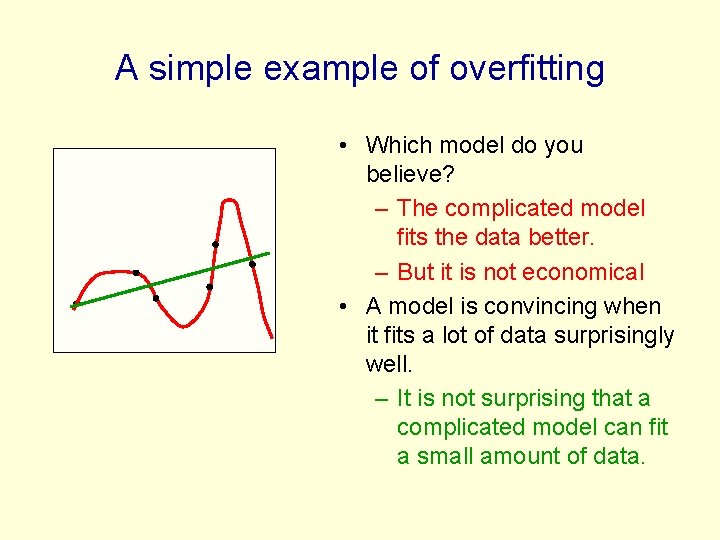
A simple example of overfitting • Which model do you believe? – The complicated model fits the data better. – But it is not economical • A model is convincing when it fits a lot of data surprisingly well. – It is not surprising that a complicated model can fit a small amount of data.