MONETARY AND MACROPRUDENTIAL POLICY WITH ENDOGENOUS RISK ASSA

MONETARY AND MACROPRUDENTIAL POLICY WITH ENDOGENOUS RISK ASSA ANNUAL MEETING, SAN DIEGO, JANUARY 5 TH, 2019 TOBIAS ADRIAN†, FERNANDO DUARTE ‡ , NELLIE LIANG ◊ AND PAWEL ZABCZYK† †INTERNATIONAL MONETARY FUND ‡FEDERAL RESERVE BANK OF NEW YORK ◊THE BROOKINGS INSTITUTION The views presented here are those of the authors and do not necessarily represent those of the International Monetary Fund or the Federal Reserve System

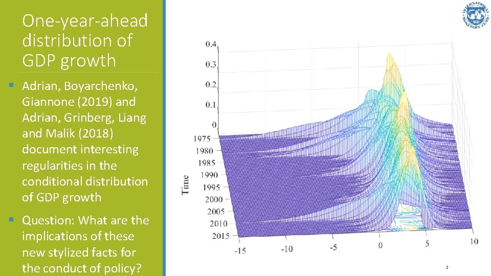
One-year-ahead distribution of GDP growth § Adrian, Boyarchenko, Giannone (2019) and Adrian, Grinberg, Liang and Malik (2018) document interesting regularities in the conditional distribution of GDP growth § Question: What are the implications of these new stylized facts for the conduct of policy? 2

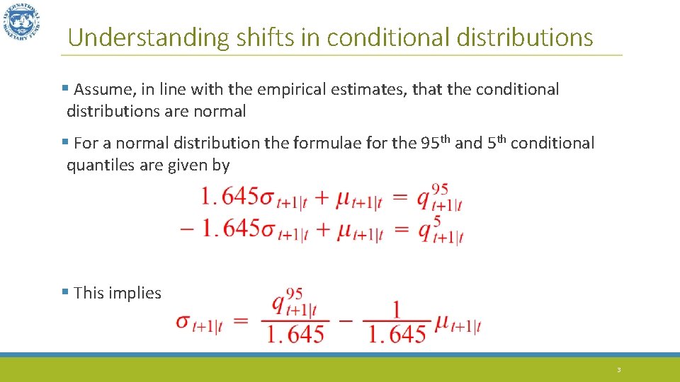
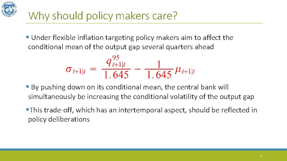
Understanding shifts in conditional distributions § Assume, in line with the empirical estimates, that the conditional distributions are normal § For a normal distribution the formulae for the 95 th and 5 th conditional quantiles are given by § This implies 3

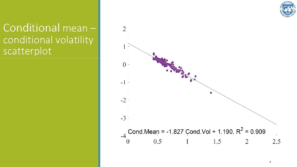
Conditional mean – conditional volatility scatterplot 4

Why should policy makers care? § Under flexible inflation targeting policy makers aim to affect the conditional mean of the output gap several quarters ahead § By pushing down on its conditional mean, the central bank will simultaneously be increasing the conditional volatility of the output gap §This trade-off, which has an intertemporal aspect, should be reflected in policy deliberations 5

Presentation Outline § Towards an NKV Model § Calibration and Fit § Policy Implications 6

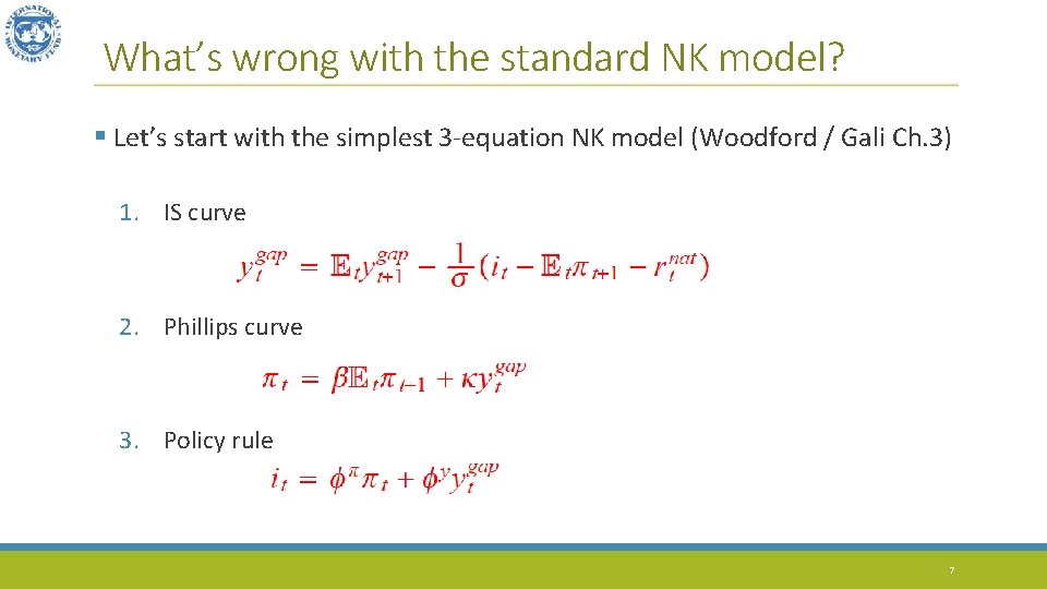
What’s wrong with the standard NK model? § Let’s start with the simplest 3 -equation NK model (Woodford / Gali Ch. 3) 1. IS curve 2. Phillips curve 3. Policy rule 7

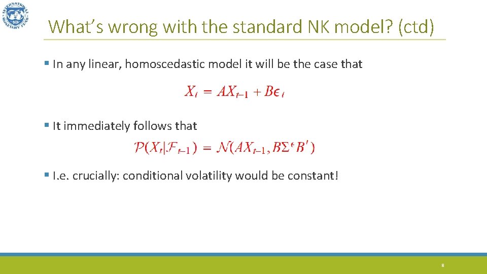
What’s wrong with the standard NK model? (ctd) § In any linear, homoscedastic model it will be the case that § It immediately follows that § I. e. crucially: conditional volatility would be constant! 8

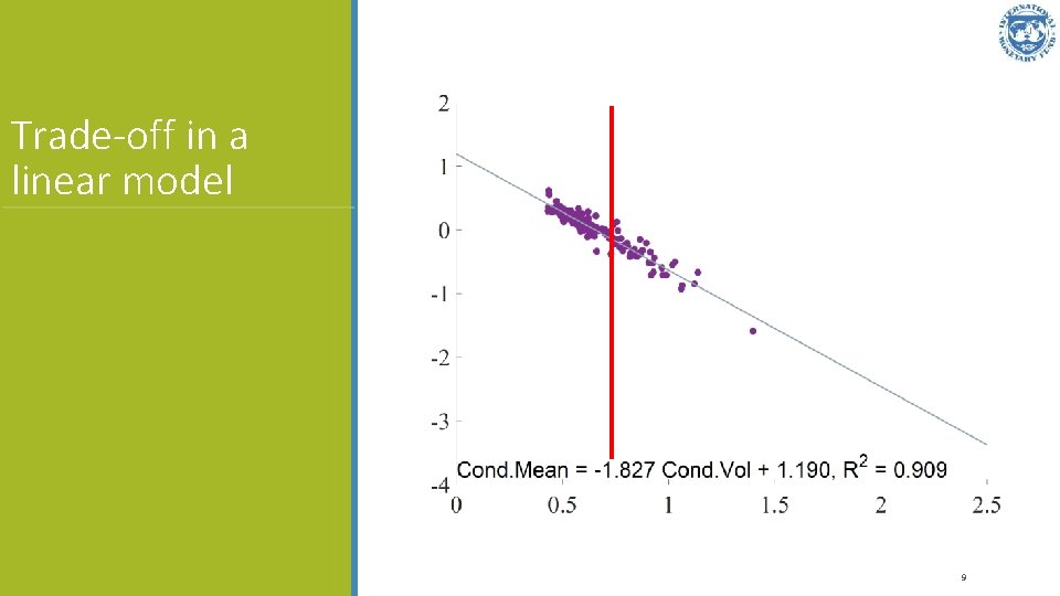
Trade-off in a linear model 9

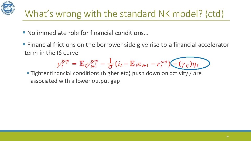
What’s wrong with the standard NK model? (ctd) § No immediate role for financial conditions… § Financial frictions on the borrower side give rise to a financial accelerator term in the IS curve § Tighter financial conditions (higher eta) push down on activity / are associated with a lower output gap 10

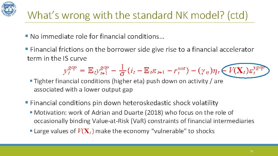
What’s wrong with the standard NK model? (ctd) § No immediate role for financial conditions… § Financial frictions on the borrower side give rise to a financial accelerator term in the IS curve § Tighter financial conditions (higher eta) push down on activity / are associated with a lower output gap § Financial conditions pin down heteroskedastic shock volatility § Motivation: work of Adrian and Duarte (2018) who focus on the role of occasionally binding Value-at-Risk (Va. R) constraints of financial intermediaries § Large values of make the economy “vulnerable” to shocks 11

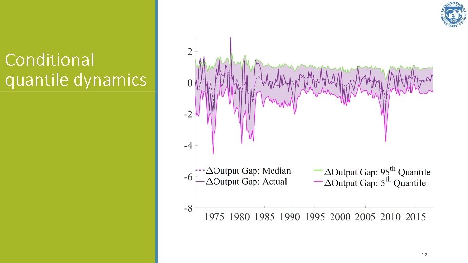
Conditional quantile dynamics 12

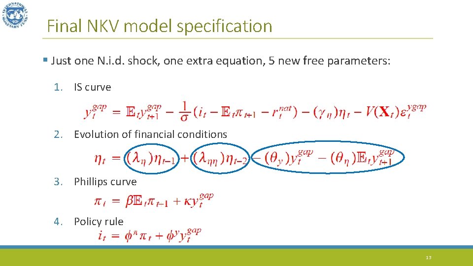
Final NKV model specification § Just one N. i. d. shock, one extra equation, 5 new free parameters: 1. IS curve 2. Evolution of financial conditions 3. Phillips curve 4. Policy rule 13

Presentation Outline § Towards an NKV Model § Calibration and Fit § Policy Implications 14

Calibration § We constrain our exercise by assuming textbook values for all NK parameters § The remaining parameters selected to match autocorrelation of ΔYgap and its cross-correlation with ETA § To focus attention on macro-financial interactions we switch off productivity and monetary policy shocks § This is in line with Adrian & Duarte (2018) who restrict attention to an IS-curve wedge 15

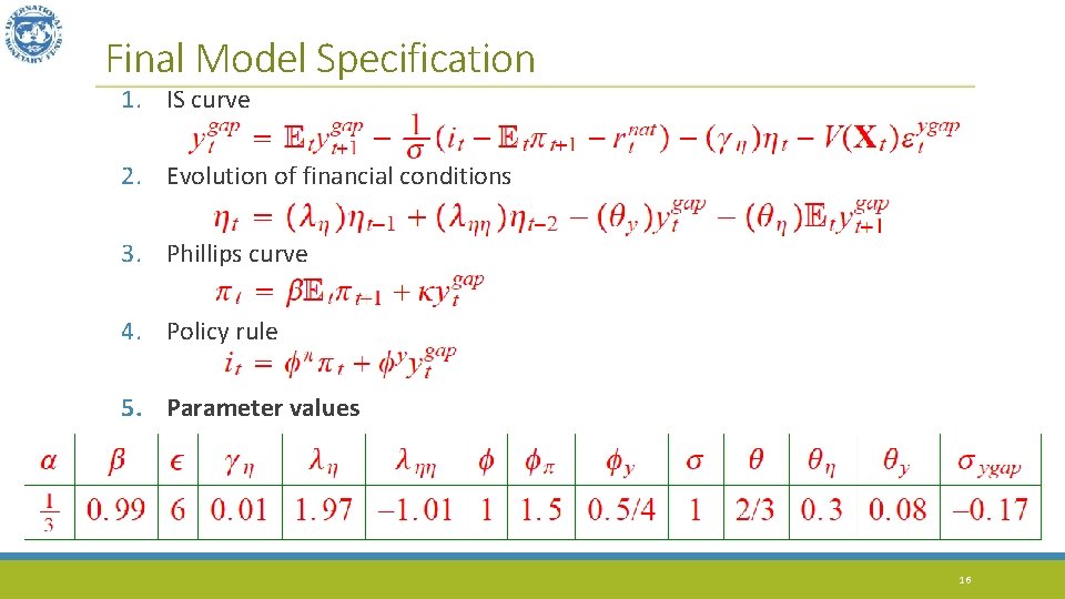
Final Model Specification 1. IS curve 2. Evolution of financial conditions 3. Phillips curve 4. Policy rule 5. Parameter values 16

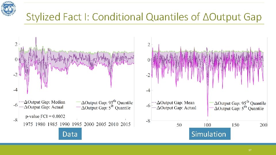
Stylized Fact I: Conditional Quantiles of ΔOutput Gap Data Simulation 17

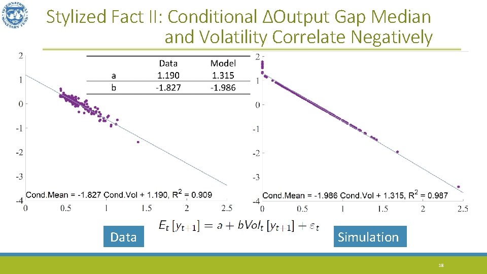
Stylized Fact II: Conditional ΔOutput Gap Median and Volatility Correlate Negatively Data Simulation 18

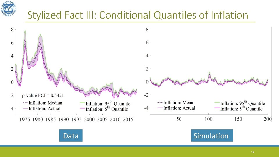
Stylized Fact III: Conditional Quantiles of Inflation Data Simulation 19

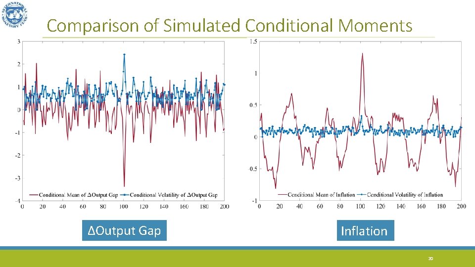
Comparison of Simulated Conditional Moments ΔOutput Gap Inflation 20

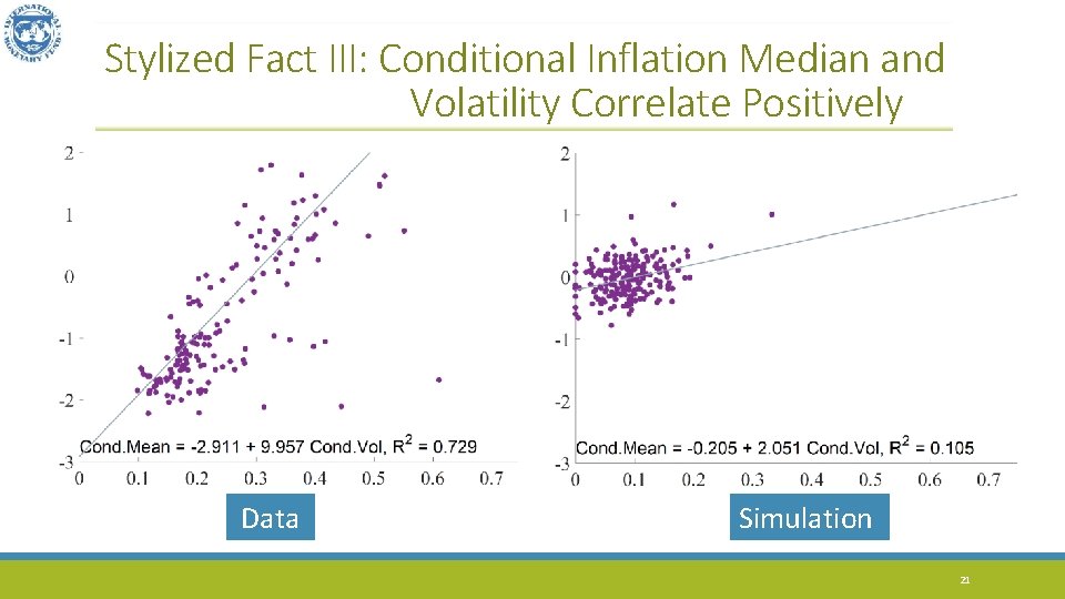
Stylized Fact III: Conditional Inflation Median and Volatility Correlate Positively Data Simulation 21

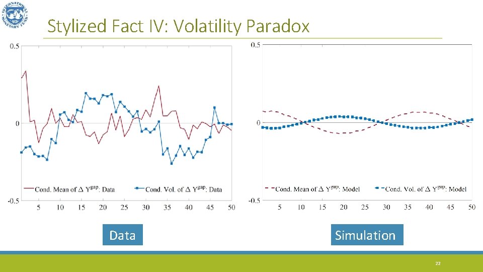
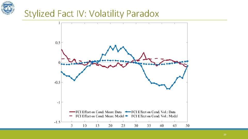
Stylized Fact IV: Volatility Paradox Data Simulation 22

Stylized Fact IV: Volatility Paradox 23

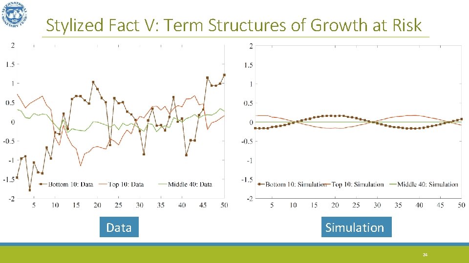
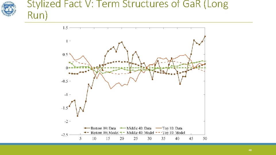
Stylized Fact V: Term Structures of Growth at Risk Data Simulation 24

Presentation Outline § Towards an NKV Model § Calibration and Fit § Policy Implications 25

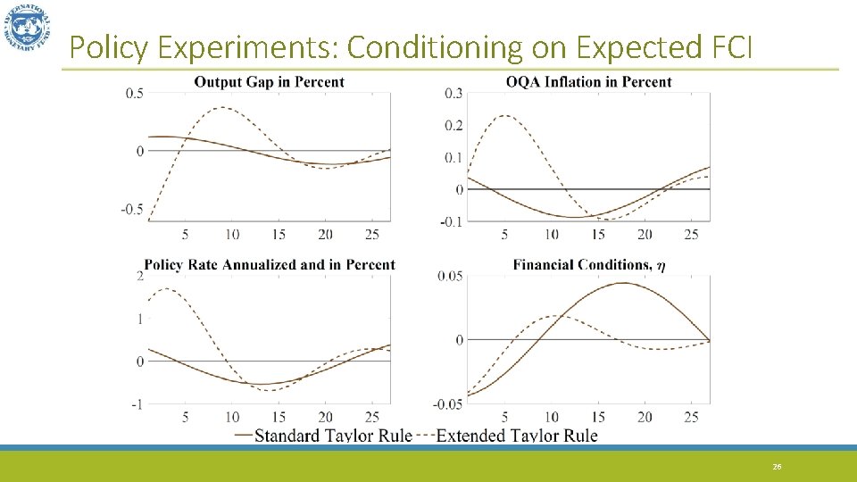
Policy Experiments: Conditioning on Expected FCI 26

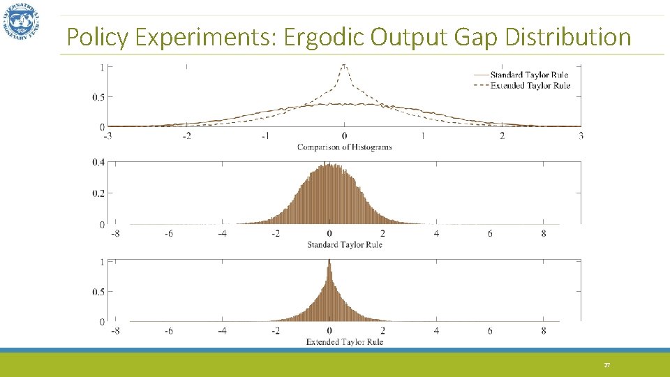
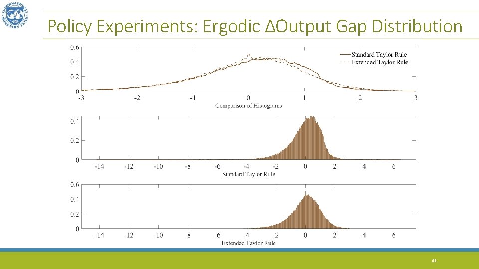
Policy Experiments: Ergodic Output Gap Distribution 27

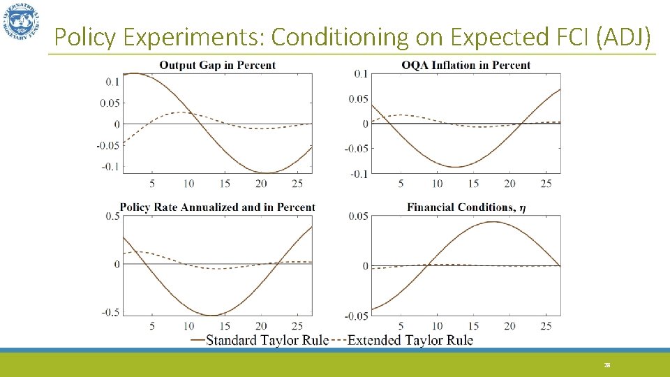
Policy Experiments: Conditioning on Expected FCI (ADJ) 28

Optimal Monetary Policy § Prior: In an NK model with a single IS curve disturbance the “divine coincidence” holds § Can sufficiently aggressive monetary policy also achieve full stabilization in the NKV model? § NO! § Once the coefficients on inflation and the output gap become too large, the model becomes unstable § In the NKV setup, monetary policy focused solely on inflation and the output gap risks destabilizing the economy! 29

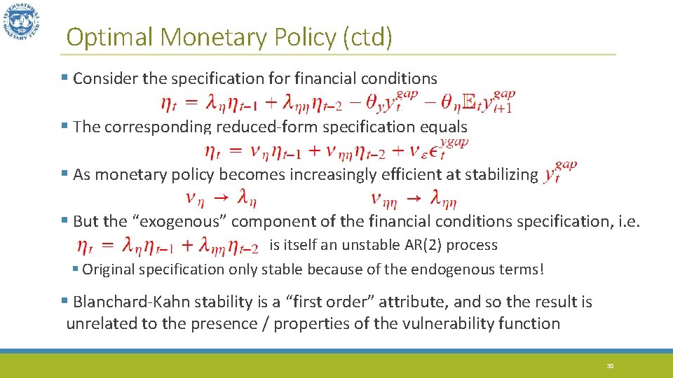
Optimal Monetary Policy (ctd) § Consider the specification for financial conditions § The corresponding reduced-form specification equals § As monetary policy becomes increasingly efficient at stabilizing § But the “exogenous” component of the financial conditions specification, i. e. is itself an unstable AR(2) process § Original specification only stable because of the endogenous terms! § Blanchard-Kahn stability is a “first order” attribute, and so the result is unrelated to the presence / properties of the vulnerability function 30

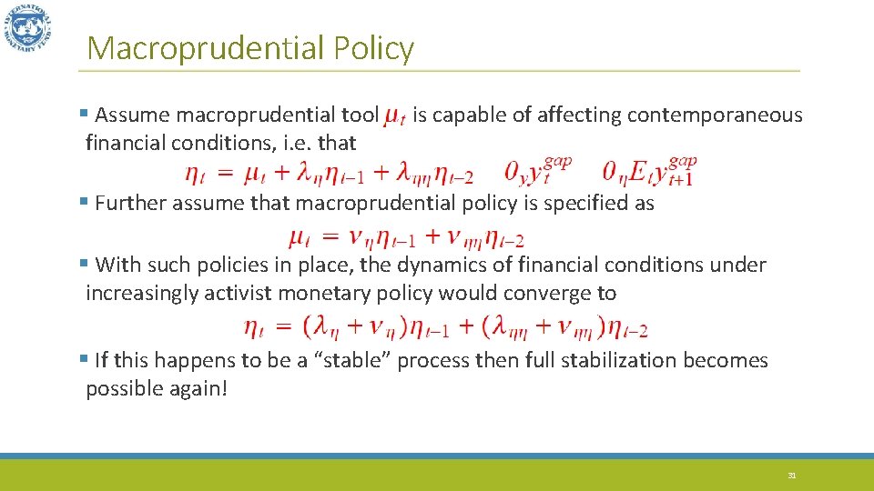
Macroprudential Policy § Assume macroprudential tool financial conditions, i. e. that is capable of affecting contemporaneous § Further assume that macroprudential policy is specified as § With such policies in place, the dynamics of financial conditions under increasingly activist monetary policy would converge to § If this happens to be a “stable” process then full stabilization becomes possible again! 31

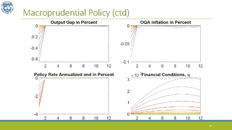
Macroprudential Policy (ctd) 32

Summary § We adapt the New Keynesian model to include “financial vulnerability” driven by movements in endogenous and forward-looking financial conditions § The resulting NKV model is calibrated to match macro-financial facts documented in Adrian, Boyarchenko and Giannone (2019) and Adrian, Grinberg, Liang and Malik (2018) § Our stylized model delivers three novel policy implications: § In contrast to the NK model, monetary policy aggressively targeting a combination of inflation and the output gap risks destabilizing the economy § Conditioning monetary policy on expected financial conditions can mitigate tail-risks § If macroprudential policy can ensure that financial conditions are “inherently stable” then a narrow mandate for monetary policy, i. e. focus purely on inflation and the output gap, can ensure full stability 33

Hidden Slides 34

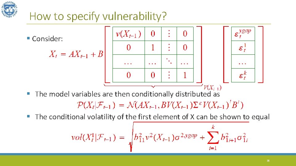
How to specify vulnerability? § Consider: § The model variables are then conditionally distributed as § The conditional volatility of the first element of X can be shown to equal 35

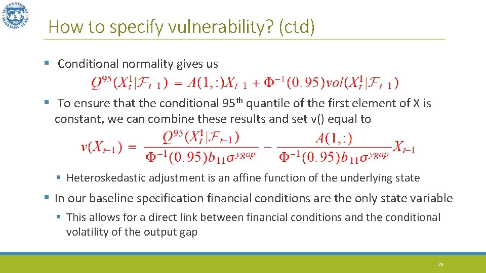
How to specify vulnerability? (ctd) § Conditional normality gives us § To ensure that the conditional 95 th quantile of the first element of X is constant, we can combine these results and set v() equal to § Heteroskedastic adjustment is an affine function of the underlying state § In our baseline specification financial conditions are the only state variable § This allows for a direct link between financial conditions and the conditional volatility of the output gap 36

What’s wrong with the standard NK model? (ctd) § NK setup inherits many properties of the RBC model – including absence of a meaningful shock propagation mechanism § If we fed the model N. i. d. shocks we would get N. i. d. processes for the output gap and inflation… § Two potential solutions: § Increase the dimensionality of the state (e. g. habits, interest rate smoothing, accelerationist Phillips curve); however, in the spirit of Ascari, Fagiolo and Roventini (2015), this doesn’t improve fit to facts in ABG (2019) § Enrich shock propagation by allowing for richer dynamics of ETA §We opt for the latter and end up with a very rich propagation mechanism 37

The price for richer propagation… § Addition of an endogenous state variable makes all analytical expressions somewhat less tractable… § E. g. equilibrium coefficient on ETA lagged (with ληη set to zero), 2 MB function text file… 38

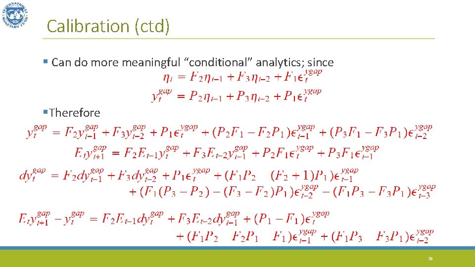
Calibration (ctd) § Can do more meaningful “conditional” analytics; since §Therefore 39

Stylized Fact V: Term Structures of Ga. R (Long Run) 40

Policy Experiments: Ergodic ΔOutput Gap Distribution 41

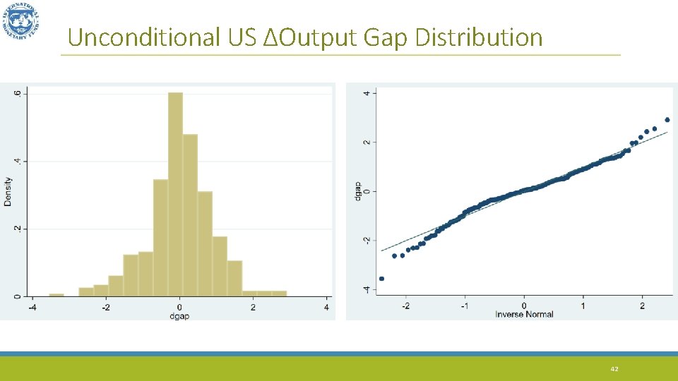
Unconditional US ΔOutput Gap Distribution 42